A Deep Dive into Positional Embeddings in Modern LLMs

This article explains how LLMs encode and process token position information by covering classic and contemporary methods like RoPE. It’s essentially a comprehensive journey where we will work through the mechanisms with visual examples, a little math, and a small PyTorch implementation. And, of course, we will then also look at how modern architectures adapt or omit explicit positional encodings.

Below, you can find a preview of which positional embedding choices are used in 2026 open-weight models. We will discuss these choices later after covering the underlying mechanisms.

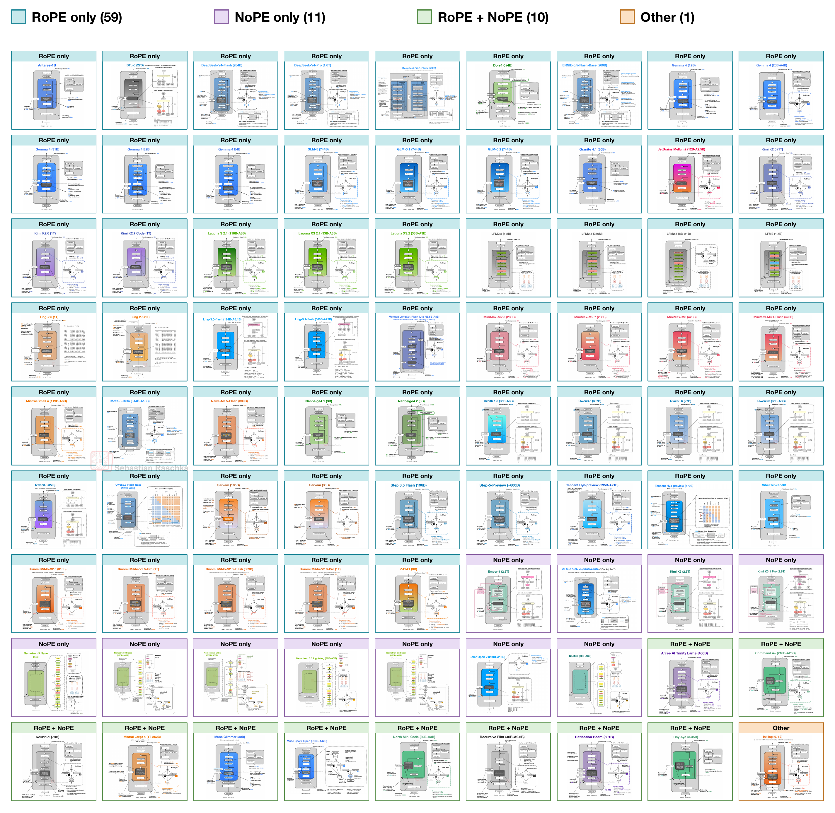Figure 1: A preview of the gallery’s 2026 architectures, grouped by positional encoding. Architecture figures taken from my LLM gallery.

But why spending so much time writing/reading about this rather minor building block? LLMs keep evolving, and as I was preparing a new article on the latest LLM architecture trends this year, I realized that I never covered the positional information methods used in LLMs in any article so far. So, instead of letting the other article get out of hand, I thought it might make sense to publish this as a standalone building block for the upcoming LLM architecture and trends analysis.

Also, over the years, many readers have asked me for a tutorial on relative positional embeddings (aka RoPE) to follow up on the learned absolute embeddings used in GPT. It’s been on my TODO list for a long time, so I finally revisited my old draft and put this walkthrough together, which will cover

• different positional methods in LLMs;
• (finally) how RoPE works;
• what methods are used by recent open LLMs.

Note that this article assumes some familiarity with basic LLM architectures and works well as a follow-up to Build a Large Language Model (From Scratch). If the concepts and computation of the attention internals, particularly query, key, and value vectors, are a little fuzzy, I recommend checking my self-attention walkthrough as a refresher:

The article is also very technical and likely too detailed for some. However, I really wanted to have this foundation out there for future articles to reference. And no worries, the next one will return to a more comfortable style.

PS: I started experimenting with Substack’s new “perks” system. As a thank-you to supporters, I’ve added image exports and metadata from the architecture gallery for you to use in your own analyses.

PPS: If you are already familiar with how position embeddings work, feel free to fast-forward to Section 6, Positional choices in modern architectures.

Note that this article may be best read in a web browser than an email client. I recommend checking out the web view here, which also has a navigation bar on the left side.

1. Where position information enters an LLM

Let’s start with the overall architecture. A tokenizer encodes the input text into token IDs. Next, the input token embedding layer of an LLM maps each of these IDs to a vector of numbers. We usually refer to these entries in that vector as “features” (similar to classic ML). The transformer blocks inside the LLM then modify these vectors using attention and feedforward layers. Lastly, the model’s output layer produces logit scores (converted into probabilities) for the next token.

The following shows this path in GPT-2 (a relatively classic LLM) and MiniMax-M3 (a more recent LLM released this year; a placeholder for most other recent LLMs). As we can see, the architectures are not too different from each other, but before we get to the positional information parts, let’s focus on the orange blocks for now (the token embedding layers) and the transformer blocks above them; the other architecture differences aren’t needed for this explanation.

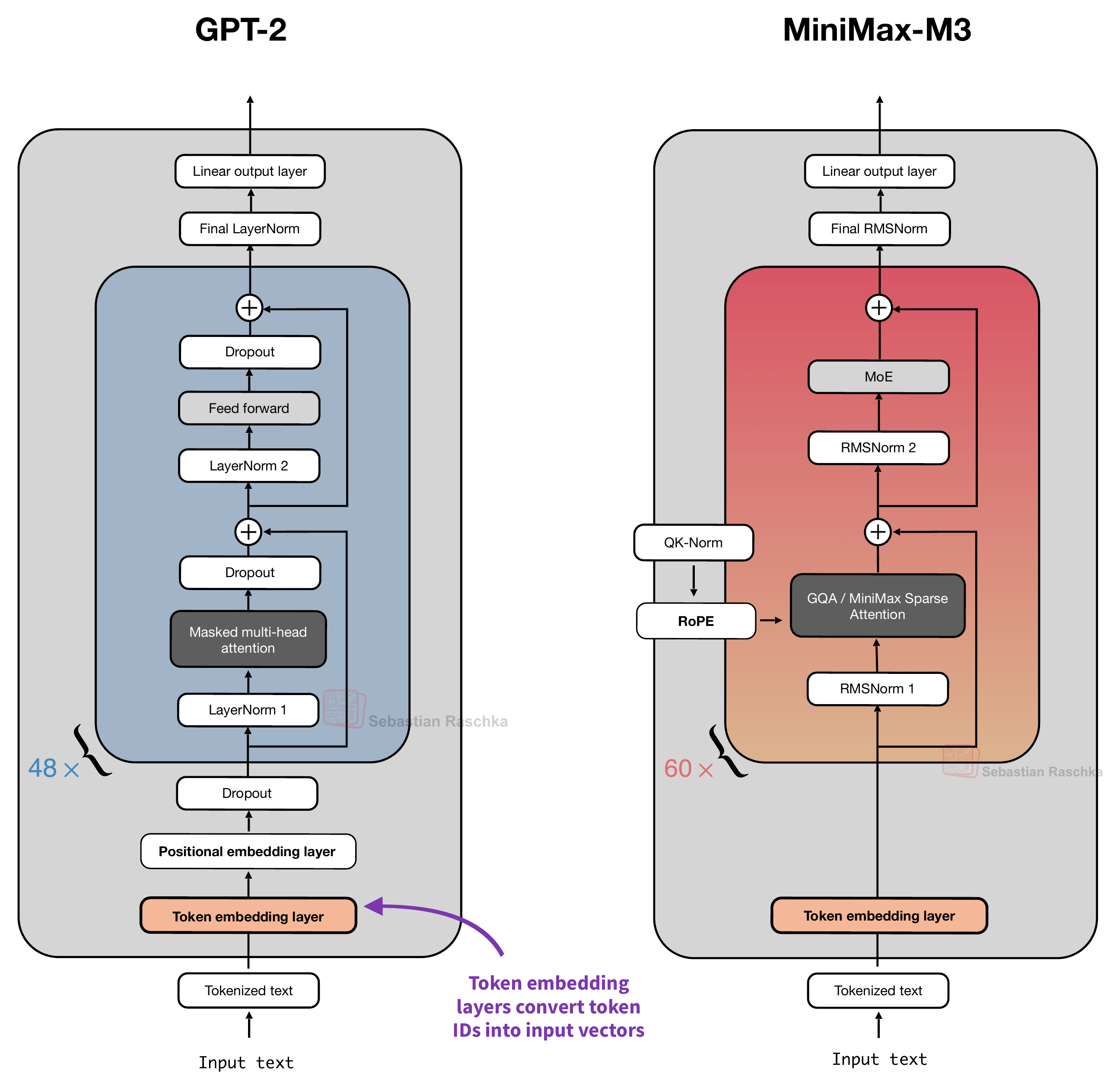Figure 2: Token embedding layers in GPT-2 and MiniMax-M3, highlighted in orange. (Side note: M3’s first three out of 60 feedforward layers are dense not MoEs.)

A token embedding layer, shown in the figure above, maps each token ID to a vector. Position information is then added afterward. Concretely, and as we will discuss in more detail later, GPT-2 adds a position vector to each token embedding before the modified embedding enters the first transformer block. On the other hand, MiniMax-M3 adds the positional information in each transformer block using a method called RoPE inside attention.

We will talk about these methods in more detail later, but first, let’s start with the big picture information explaining why explicit positional information is added or needed.

1.1 Why add positional information?

Consider the following two input sentences as a simple example:

1. “The red fox jumps over the gray fox.”
2. “The gray fox jumps over the red fox.”

Changing the word order changes which fox does the jumping, as illustrated in the following figure.

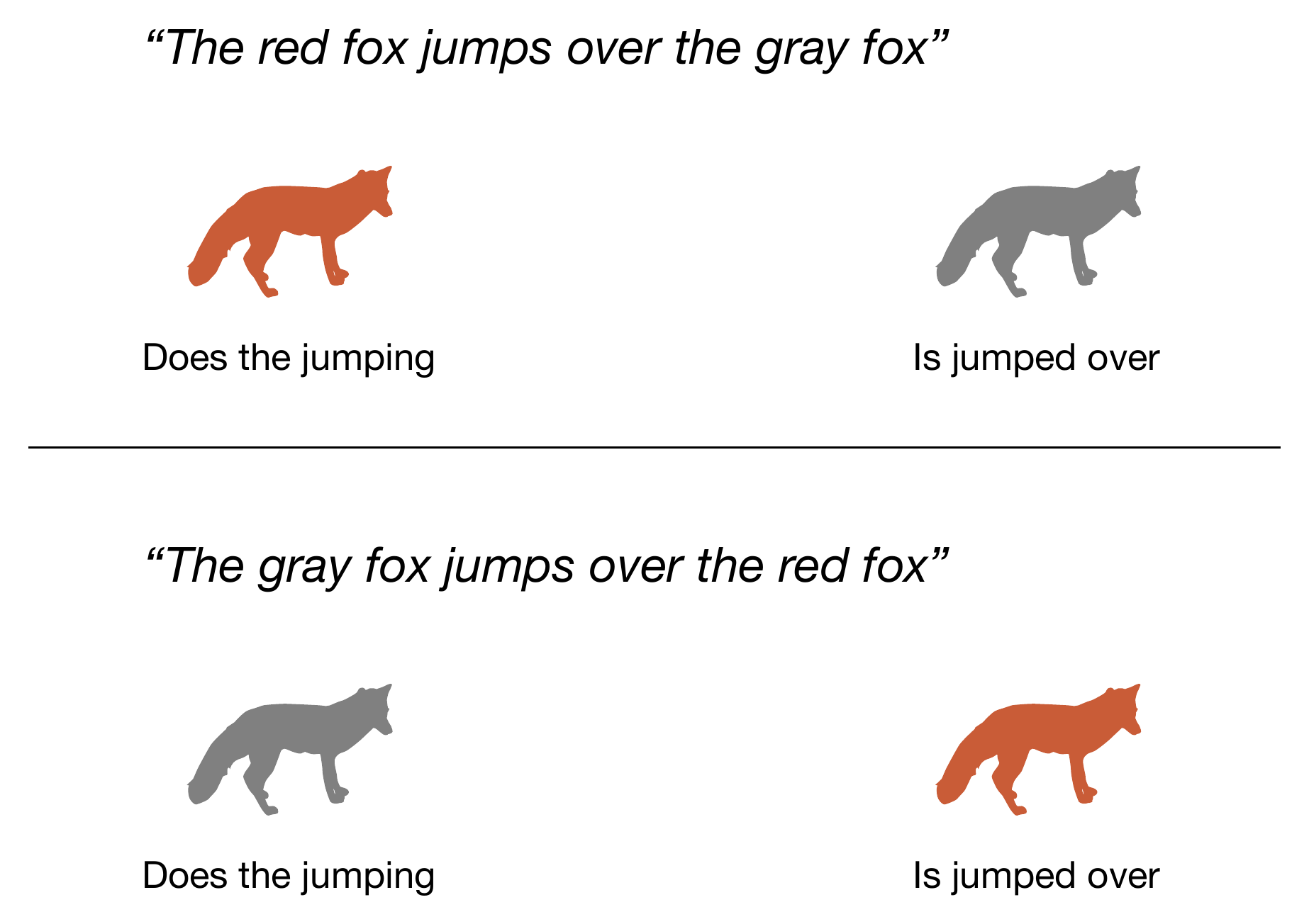Figure 3: Changing the word order changes which fox jumps.

For the examples in this article, we will treat each word as one token for simplicity. (As you know, real tokenizers can split words into smaller subword tokens.) The first sentence then has eight token positions, from 0 through 7.

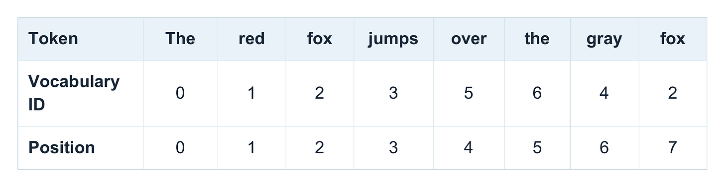
Figure 4: Token IDs and positions in the toy sentence.

# Assume the following small vocabulary.
# Real vocabularies typically have 50k to 200k entries
vocab = {
    "The": 0,
    "red": 1,
    "fox": 2,
    "jumps": 3,
    "gray": 4,
    "over": 5,
    "the": 6,
}

(If you are interested in how vocabularies are built, check out my tokenizer materials on GitHub.)

Note that “fox”, which appears twice in the input sentence, gets the same token ID 2 in both cases. And since they both have the same token ID, irrespective of the position in the input sentence, they would get the same embedding vector from the embedding layer.

Now, let’s consider a regular self-attention mechanism with no positional encoding (and no causal mask), where every input token can attend to every other token in the input. In this scenario, swapping any two words, like “red” and “gray”, would still result in the same embeddings and attention scores between each token pair.

GPT-style models do use a causal (autoregressive) mask, which restricts each token to itself and earlier tokens. Interestingly, this causal mask gives the computation some implicit order information. In our example, “jumps” can attend to “red” in the first sentence and “gray” in the second. So, a causal LLM can theoretically already distinguish these sentences even without explicit positional embeddings. (We will return to this idea later when discussing the “NoPE” concept.)

Nonetheless, GPT-2 and most newer LLMs include explicit positional information because it gives attention a direct signal about positions. That’s because even though the causal mask determines which tokens are accessible and provides implicit order information, it doesn’t distinguish a separation of one position from a separation of ten, for example. So, explicit positional methods are still useful (or even essential), since they supply that information.

If this all sounded confusing, don’t worry, it was more meant as an overview, and we will step through these concepts a bit more slowly in the remaining article.

2. Adding a position vector to each token embedding

We briefly talked about implicit positional information through causal attention masks (and we will revisit this again in more detail later). However, we now switch gears and talk about the explicit ways to add positional information.

The perhaps simplest and most direct (but not “cheapest”) approach is to give each sequence position its own vector. We add that vector to the token embedding, so the resulting, modified embedding vector is then passed to the first transformer block. This exact procedure is discussed in the following subsections.

2.1 Learned absolute position embeddings in GPT-2

To illustrate the use of an explicit, learned positional vector to the input embeddings, let’s consider GPT-2 as a concrete example. GPT-2 learns a table of position vectors during training. The following figure illustrates where these vectors are used in the architecture, that is, immediately after the token embedding lookup and before the first transformer block.

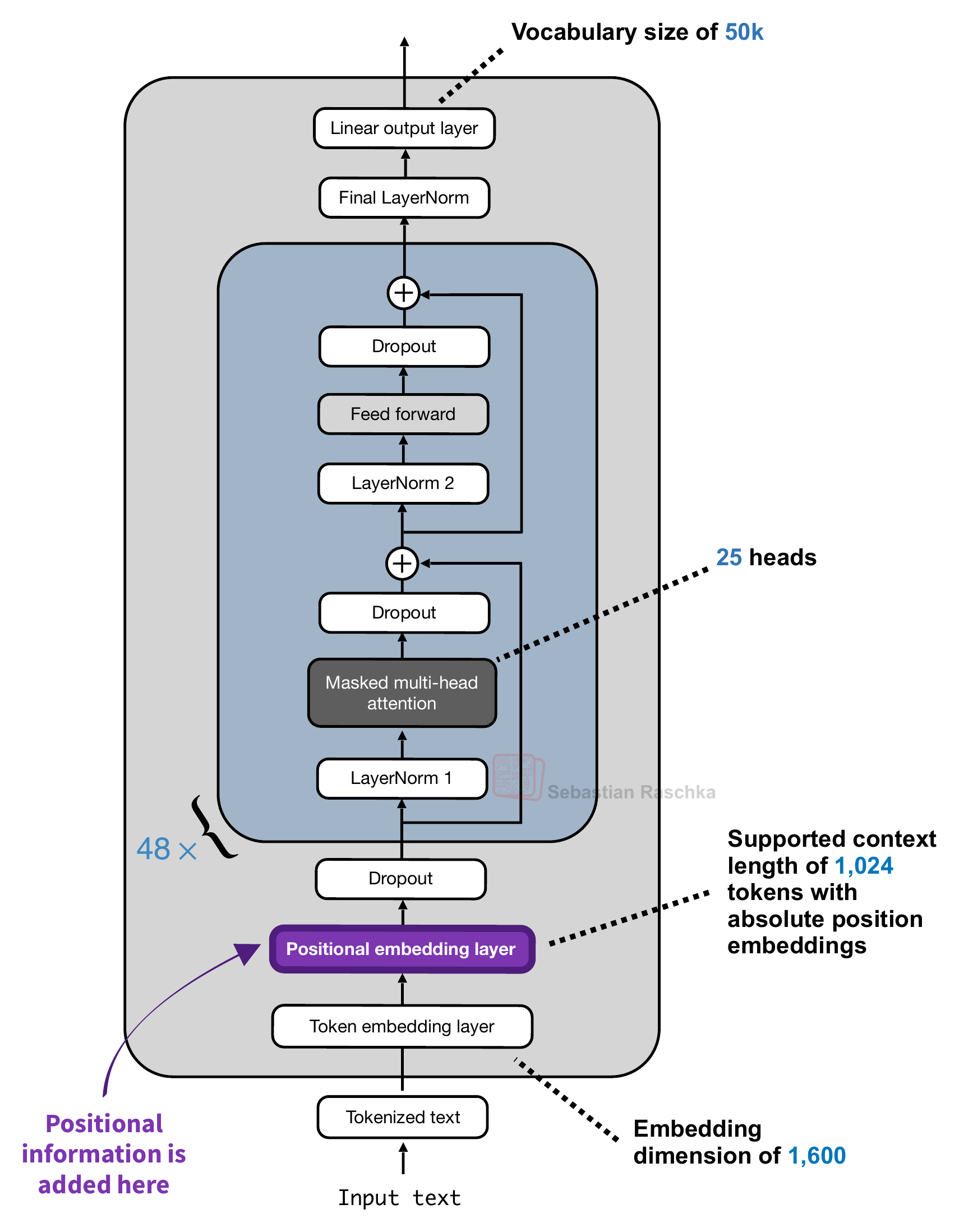Figure 5: GPT-2 adds absolute position information before the transformer blocks, as highlighted in purple. The dimensions shown are for GPT-2 XL.

The positional embedding layer depicted in the figure above follows the same implementation as the token embedding layer, i.e., they have exactly the same output dimensions so that the resulting input vectors can be added to each other. The code below shows that with an excerpt of a GPT-2 code implementation:

class GPTModel(nn.Module):
    def __init__(self, cfg):
        super().__init__()
        self.tok_emb = nn.Embedding(cfg["vocab_size"], cfg["emb_dim"])
        self.pos_emb = nn.Embedding(cfg["context_length"], cfg["emb_dim"])
        self.drop_emb = nn.Dropout(cfg["drop_rate"])

        self.trf_blocks = nn.Sequential(
            *[TransformerBlock(cfg) for _ in range(cfg["n_layers"])])

        self.final_norm = LayerNorm(cfg["emb_dim"])
        self.out_head = nn.Linear(
            cfg["emb_dim"], cfg["vocab_size"], bias=False
        )

    def forward(self, in_idx):
        batch_size, seq_len = in_idx.shape
        tok_embeds = self.tok_emb(in_idx)
        pos_embeds = self.pos_emb(torch.arange(seq_len, device=in_idx.device))
        x = tok_embeds + pos_embeds  # Shape [batch_size, num_tokens, emb_size]
        x = self.drop_emb(x)
        x = self.trf_blocks(x)
        x = self.final_norm(x)
        logits = self.out_head(x)
        return logits

And in mathematical terms, we can write it as follows. Let m be a position index and xm the token ID at that position. The input to the first block is

Here,

• Etoken is the embedding layer,
• Pm is the position info vector selected by m,
• and hm is the resulting summed embedding and position vector.

The two vectors have the same width, so we add their entries element-wise. Figure 6 below shows this visually with a small numerical example.

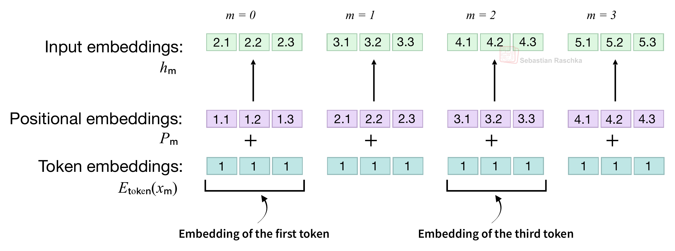Figure 6: Token and position embeddings are added element-wise. (I am following the convention here that neural network diagrams are usually read from bottom to top.)

In the figure above, at position 0, adding the token embedding [1, 1, 1] to the position embedding [1.1, 1.2, 1.3] gives [2.1, 2.2, 2.3]. By the way, the values in the figure are chosen to keep the illustration simple; in a real example, both embedding layers (tables) are initialized with small random values and learned during training.

So, what we covered in this section is a so-called absolute positional method because the positional embedding Pm depends on the token’s own position m. In the previous example sentence, the two “fox” tokens have initially the same token embeddings, but because we are adding different positional vectors P2 and P7, they have different values before they enter the first transformer block. And consequently, the query, key, and value vectors inside the attention mechanisms then also receive representations that already include position information.

Note that the original GPT-2 implementation has 1,024 learned position vectors. This means it only works with inputs with 1024 or fewer tokens. If we want to extend the context window, we would have to extend this embedding table. And since the embedding table (layer) is updated like any other layer during training, the context length would have to be decided before the training starts.

Extending the context would be very expensive since the table can become very large. For example, in the case of GPT-2 Medium, the positional embedding layer weights only make up 0.30% of the total weights at 1,024 positions. However, if we increased the context length to a nowadays common 100k range, they would make up >22% of the total model weights, which would be very uneconomic.

2.2 Fixed sinusoidal position encodings in the original transformer

The original “Attention Is All You Need” transformer from 2017, which predates GPT, uses the same addition mechanism, but computes its position vectors with fixed sine and cosine functions. Figure 7 below shows this addition before both the encoder and decoder stacks. The encoder processes the input sequence, and the decoder generates the output sequence. (The reason why it’s introduced here is that the sine and cosine functions will become relevant again later when discussing RoPE.)

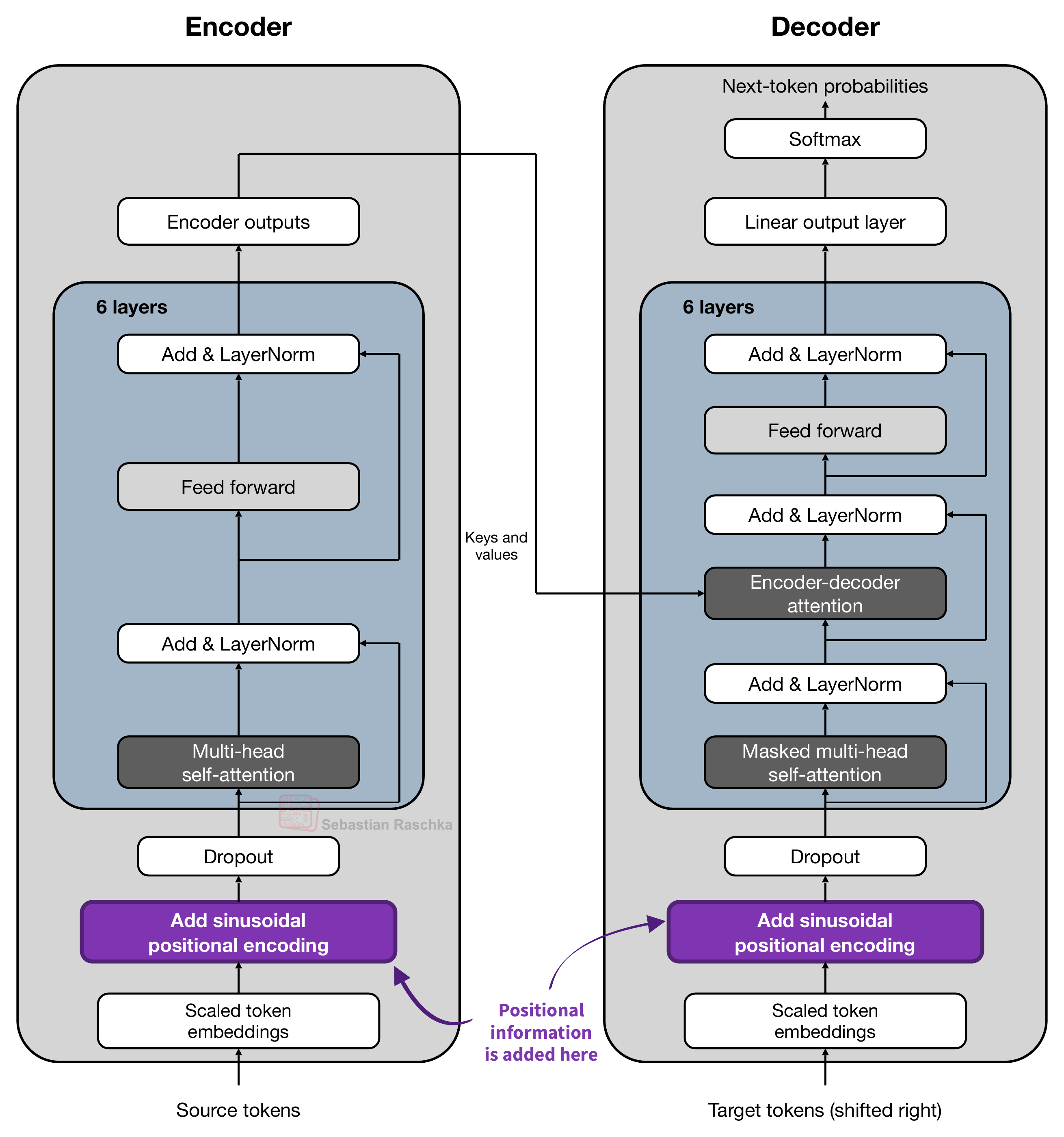Figure 7: Sinusoidal position encodings added to the token embeddings as highlighted in purple.

The original transformer also scales its token embeddings by √(dmodel) before adding the position vectors, where dmodel is the embedding width.

So, while GPT-2 in the previous section had the formula

the formula used in the original transformer (depicted in Figure 7) is:

This scaling by √(dmodel) is a minor technical detail, but for those who are curious, the motivation behind this scaling factor is not explained in the transformer paper, but as I discussed with colleagues on a Twitter thread many years ago, it’s likely to put the token embeddings and sinusoidal positional encodings on comparable numerical scales at initialization, so the position vectors don’t dominate the sum when we add them.

In the GPT-2 case, this scaling wasn’t necessary because the original GPT-2 code initialized the token embeddings to have an initial standard deviation of 0.02 and the position embeddings to have an initial standard deviation of 0.01 so that they were already roughly on the same scale.

Now, the more interesting point is how the position embeddings Pm are computed.

Concretely, each position vector has the following entries:

As before, m denotes the position. The index i indexes a pair of features within the vector.

Here, a feature is one number in the position vector. For example, let’s assume we have a small vector with 8 values (dmodel = 8) that has entries numbered 0 through 7. (In the original paper this was 512 for the small model and 1024 for the bigger model, instead of 8, but that would be hard to visualize.) We group these into four pairs so that i goes from 0 through 3.

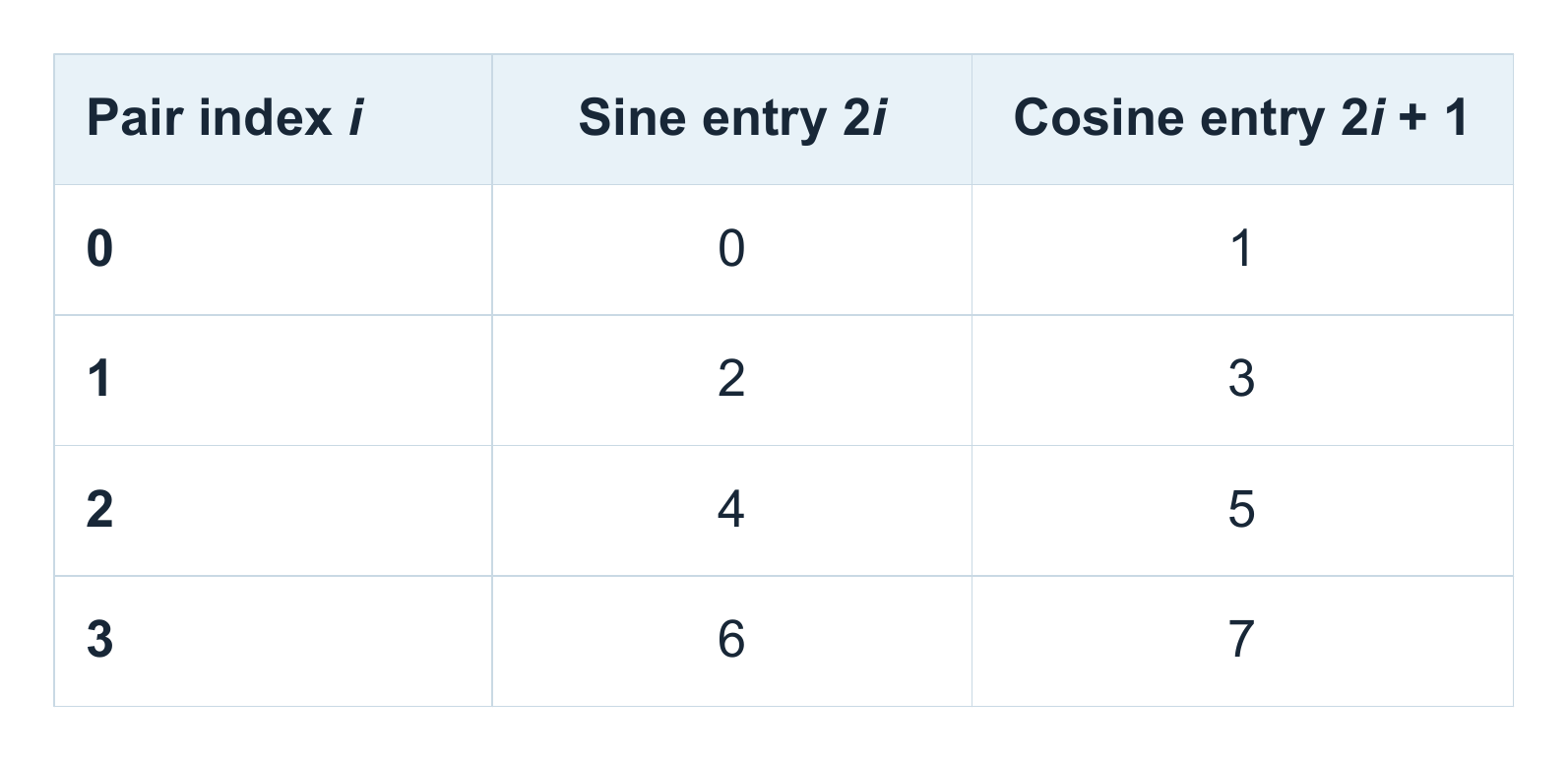Figure 8: Sine and cosine entries for each feature pair.

Here, the indices 2i and 2i + 1 select the two entries corresponding to pair i.

As shown in the equation earlier, the angle at position m, which is then fed into the sine or cosine functions to obtain Pm, 2i or Pm, 2i + 1, respectively, is computed as follows:

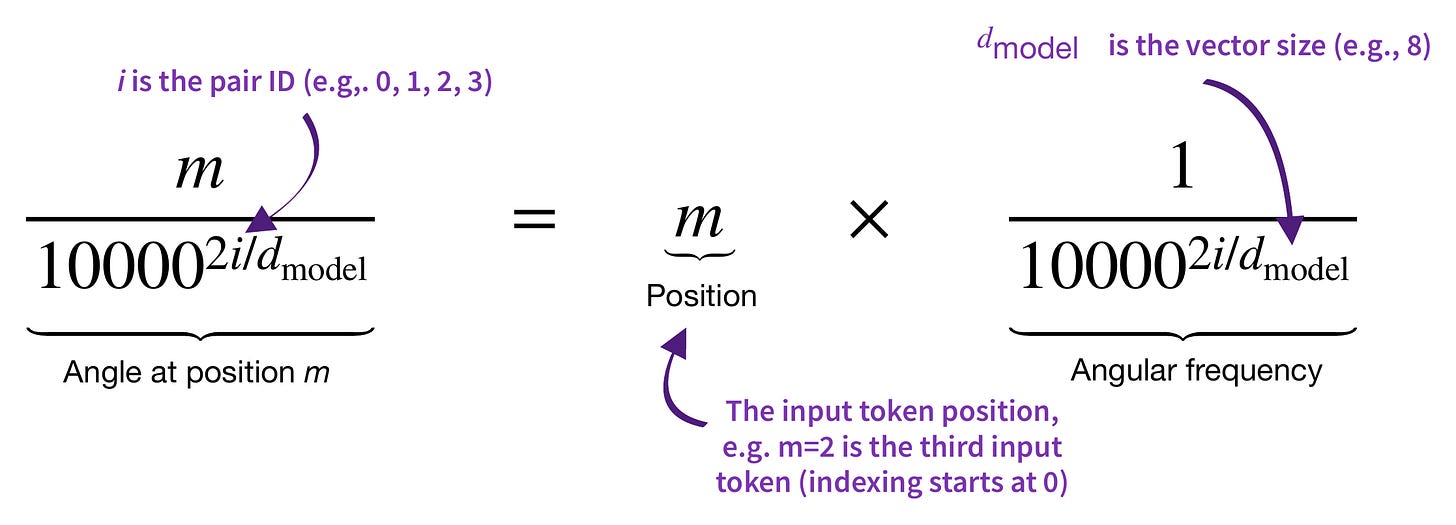
Figure 9: The angle inside sine and cosine is the token position multiplied by the pair’s angular frequency.

Figure 10 shows this calculation for all four pairs of our 8-feature example at position m = 2.

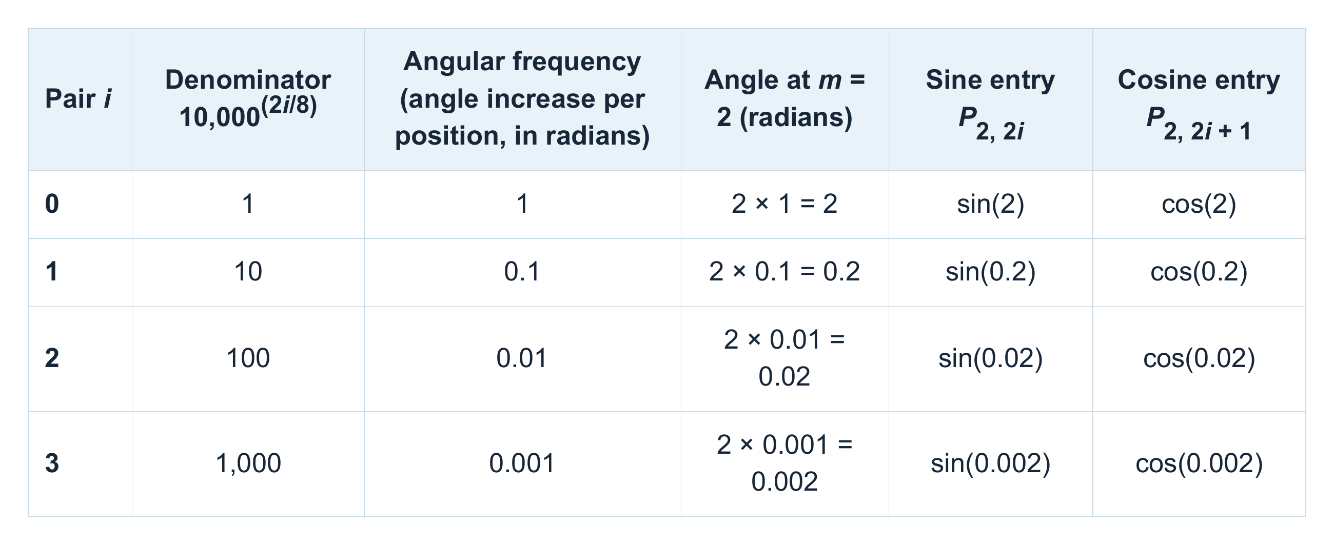Figure 10: The four sine and cosine pairs at position 2.

For an eight-feature embedding, the four frequencies are 1, 0.1, 0.01, and 0.001 radians per position. At position 2, the first pair in row 1 is (sin 2, cos 2) ≈ (0.909, −0.416).

The second pair, in row 2, changes more slowly, giving (sin 0.2, cos 0.2) ≈ (0.199, 0.980).

The figure below visualizes the sine and cosine calculations for different pairs, which are then collected in a position vector.

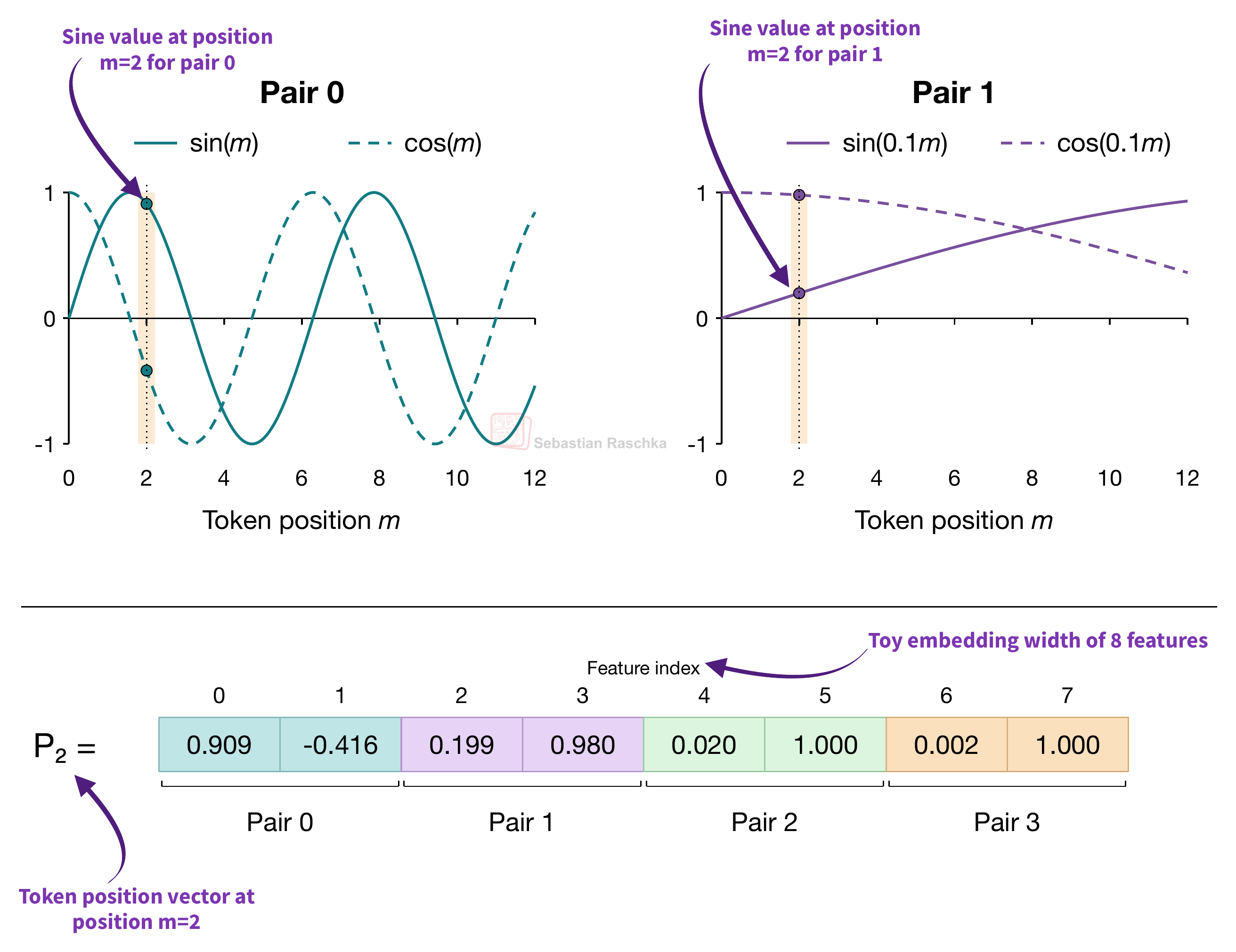Figure 11: Sampling sine and cosine functions to form a position vector.

In short, this method is a (more complicated) alternative to obtaining positional embedding vectors compared to the GPT-2 method discussed earlier.

Similar to the GPT-2 embeddings, these are also absolute embeddings because each vector is computed from its own position. However, in contrast to the GPT-2 approach, the sine and cosine functions stay fixed during training. (Also, they can be extended and evaluated beyond the training positions, like beyond the context length of 1024, although that alone doesn’t guarantee that the model will perform well there, because it hasn’t seen those during training.)

To summarize, Figure 12 below compares the two ways of obtaining a position vector we discussed so far.

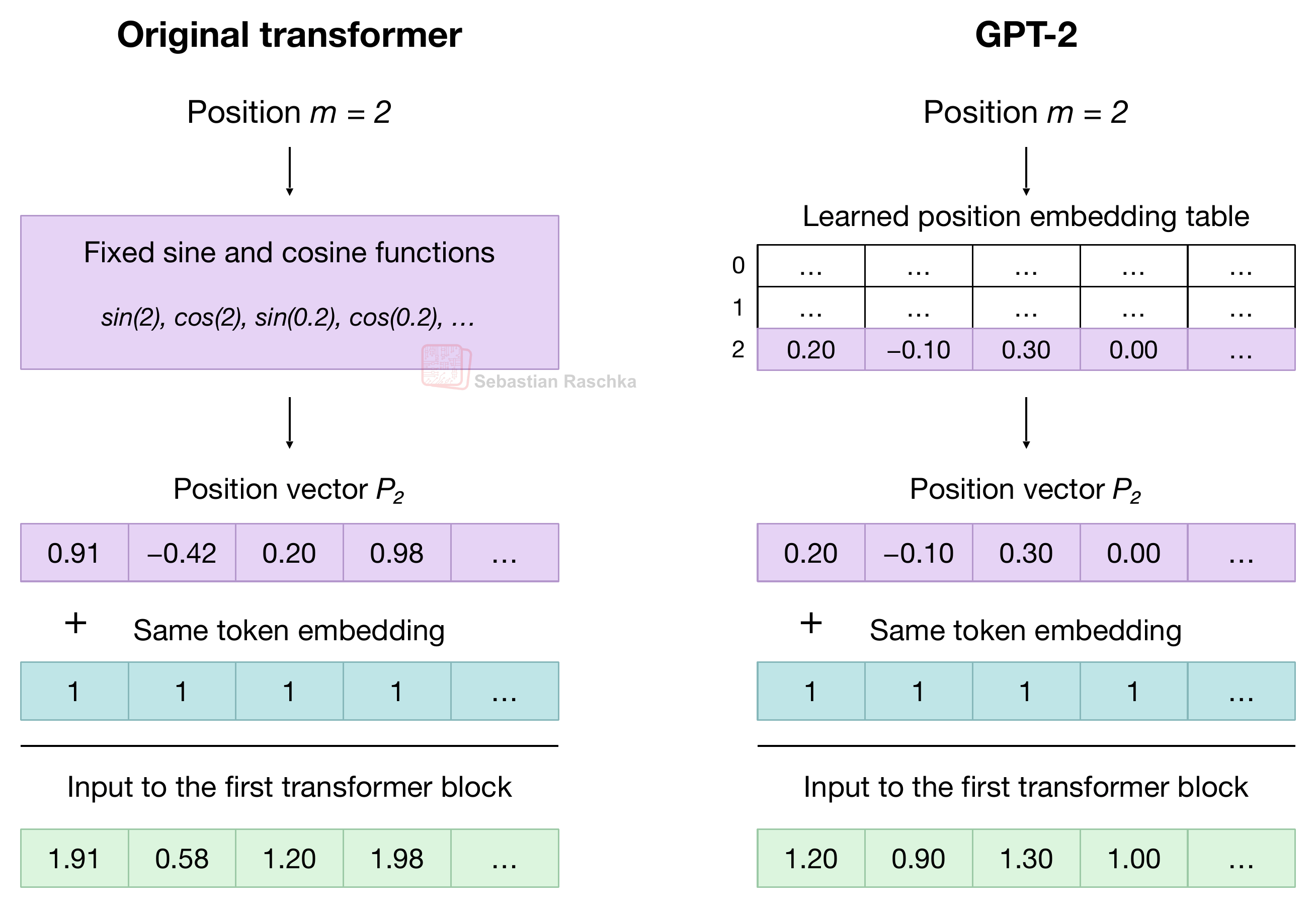Figure 12: Fixed sinusoidal and learned absolute positional embeddings.

This sinusoidal method may look like an overly complicated way to obtain positional embeddings, however, understanding it will be useful when talking about RoPE in the next section.

Also, there is some rationale behind it. The authors chose sine and cosine because they make the shifting by a certain offset gives a certain deterministic difference. For example, the difference between position 2 to 5 and the difference between 102 to 105 is both 3, which then results in the same rotation.

According to the Attention Is All You Need paper:

“...easily learn to attend by relative positions, since for any fixed offset k, PEpos + k can be represented as a linear function of PEpos.”

Or in less technical terms, the authors hypothesized that this property would make it easier for attention to learn relationships such as “three tokens earlier.”

Figure 13 below illustrates this for one sine/cosine pair. A rotation is a linear transformation, and both three-position shifts use the same rotation.

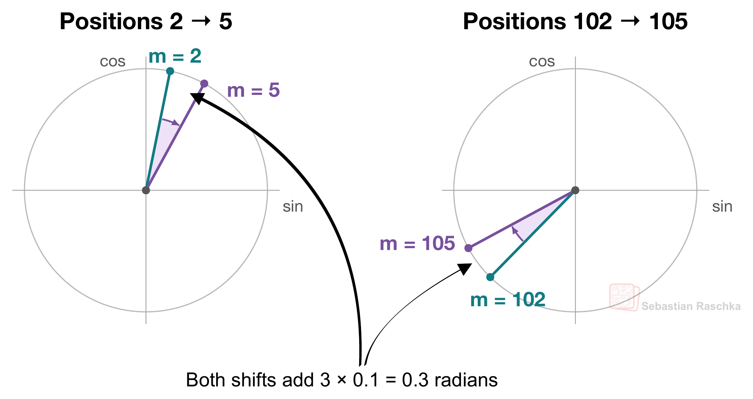Figure 13: For a pair with angular frequency 0.1 radians per position, a shift of three positions always rotates the pair by 0.3 radians.

3. Encoding relative position with RoPE

So, the sinusoidal method above is still considered an absolute positional encoding because the vector added to each token embedding represents that token’s position counted from the start of the sequence.

As shown in the previous figure, for example, tokens at positions 2 and 5 receive the position vectors P2 and P5. If we move those tokens to positions 102 and 105, they’re still three positions apart. But each token gets a different position vector because its absolute position m has changed.

So their attention score can change even when the token embeddings stay the same. The sinusoidal structure still gives the model a way to learn relative relationships.

Anyways, RoPE, which we will discuss below, builds this relative relationship directly into the attention calculation. RoPE, which Su et al. introduced in the 2021 RoFormer paper, stands for Rotary Position Embedding and is considered a relative position method.

3.1 Moving the rotation inside attention in RoPE

In attention, each token’s current representation is projected into a query, a key, and a value vector. Query-key dot products determine attention scores. After masking and softmax, the resulting weights determine how the value vectors are mixed. For a refresher, see my Understanding and Coding Self-Attention, Multi-Head Attention, Causal-Attention, and Cross-Attention in LLMs article:

RoPE uses the token’s position to rotate its query and key vectors before their dot product. The value vectors bypass this rotation. Figure 14 below shows an overview of where RoPE is applied in a relatively recent MiniMax-M3, where QK-Norm normalizes queries and keys before RoPE.

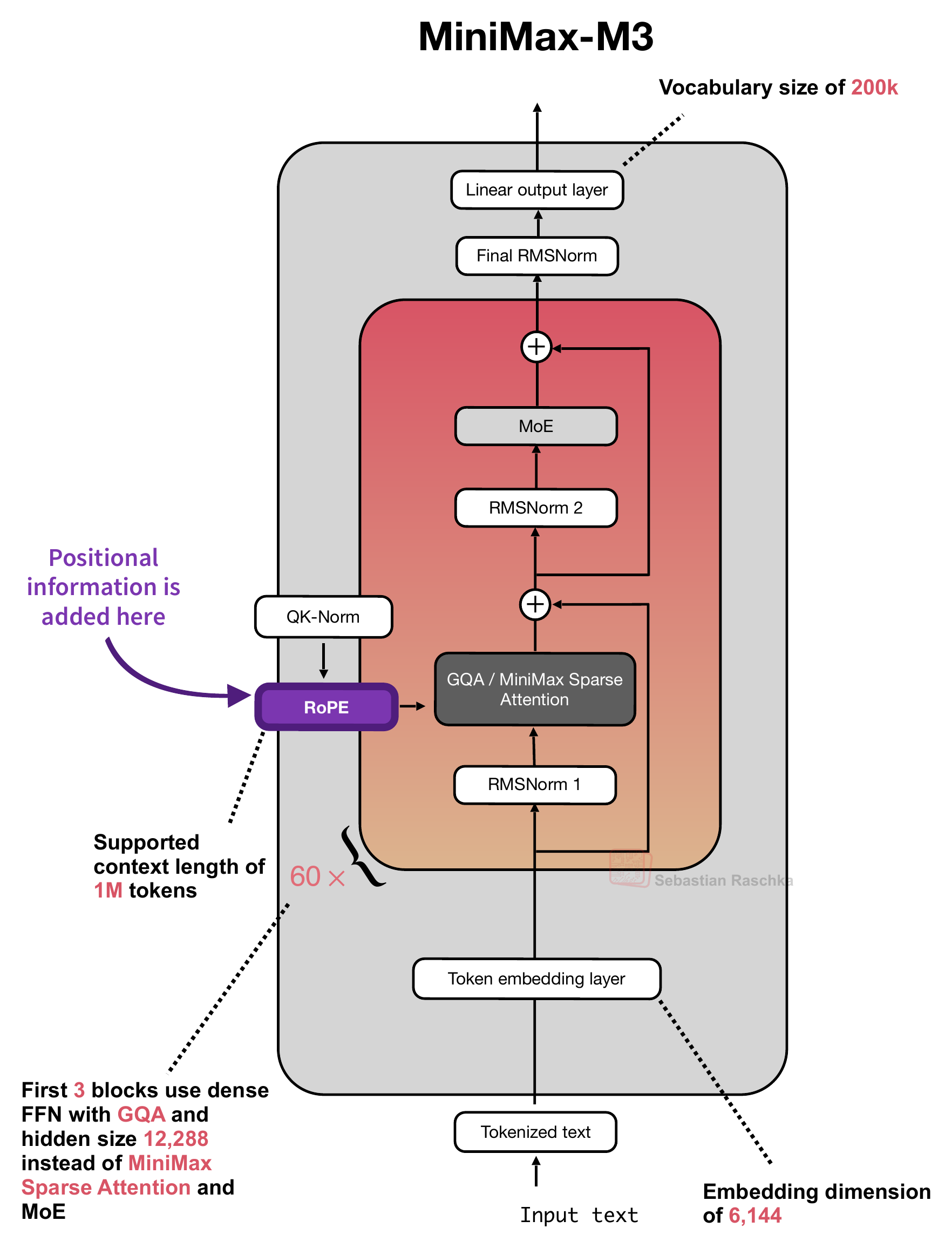Figure 14: MiniMax-M3 applies RoPE to queries and keys inside attention.

As shown in the figure above, the LLM architecture has no explicit position vector added alongside the initial token embedding. Its explicit position signal is injected inside attention instead.

Side note: MiniMax-M3 rotates only part of each query and key head, a variation known as “partial RoPE” that we will cover later in Section 6.1. But to understand the basic RoPE operation first, let’s walk through the method step by step using a small example.

3.2 From token representations to feature pairs in RoPE

Attention usually divides its query, key, and value features into multiple heads, which are processed in parallel. Hence, the full mechanism is usually called Multi-head Attention (note that Grouped Query Attention also uses multiple heads). Here, each attention head computes its own attention scores and weighted sums. RoPE then acts on pairs of numbers within each query and key head.

To make this concrete, Figure 12 below follows a token representation through the learned query and key projections, which are computed via the weight matrices WQ and WK. In this toy example, each projection produces 16 features, which are reshaped into two heads with eight features each. In the figure below, every small cell contains one scalar feature, meaning one numerical entry in a vector (the numbers are not shown due to space reasons).

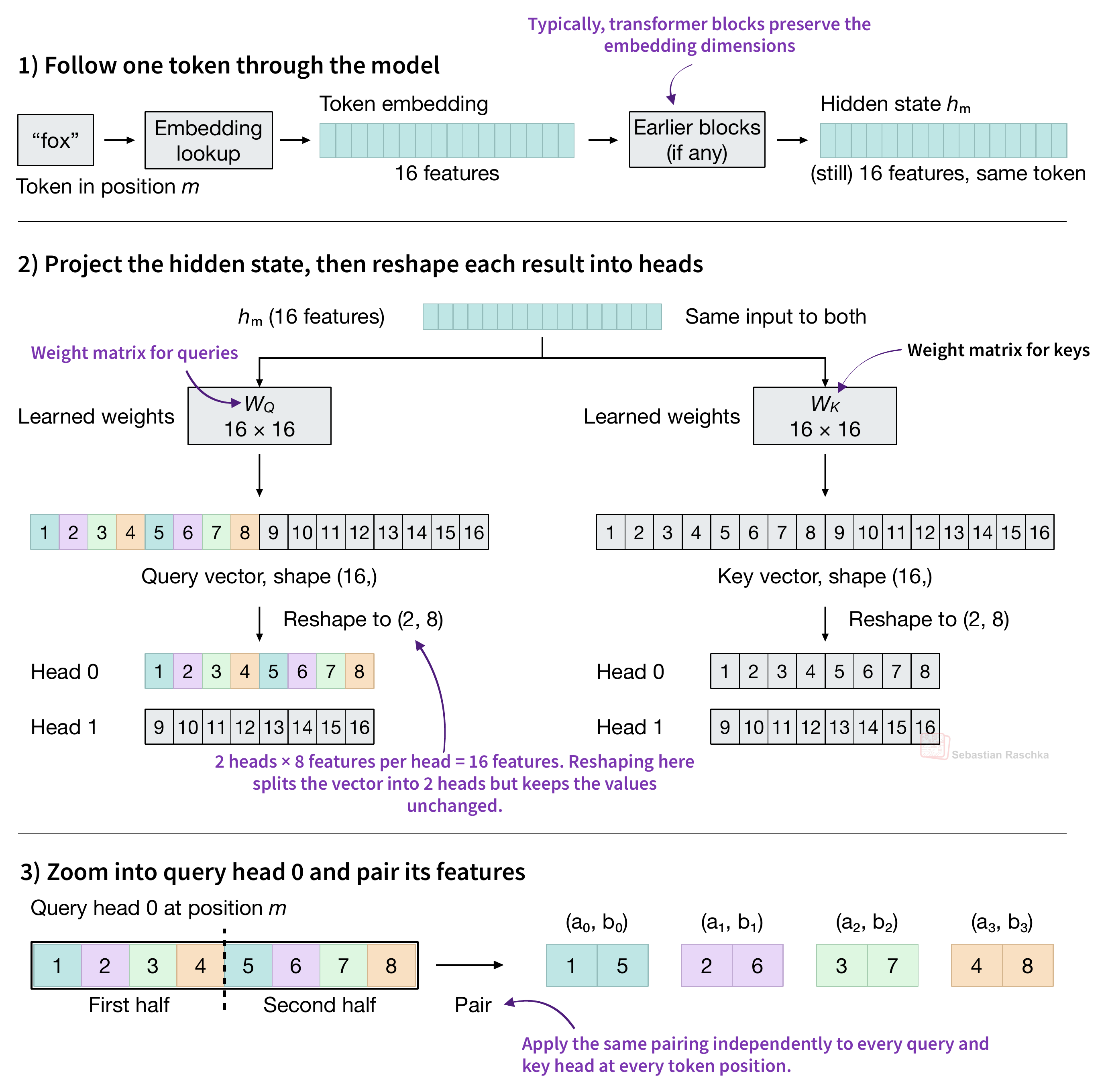Figure 15: Projecting a hidden state, reshaping into heads, and pairing features for RoPE.

For the first eight-feature head, [1, 2, 3, 4, 5, 6, 7, 8], we pair each feature in the first half with the corresponding feature in the second half. This gives (1, 5), (2, 6), (3, 7), and (4, 8). This split-half convention is used in LLM implementations, including my Qwen3 implementation. (We will compare it with the original, alternative adjacent-feature pairing method later after implementing the basic operation.)

Each pair gets a rotation angle determined by the token position m and that pair’s frequency θi. The corresponding query and key pairs use the same frequency. Figure 16 below shows how we rotate the pairs, put the updated features back in their original locations, and compute the query-key dot product.

Figure 16: Pairwise rotations produce the rotated query and key vectors used to compute attention scores.

The next section will walk through the figure(s) a bit more slowly.

3.3 Rotating one pair in RoPE

For the following example, we’ll use the same two positions as before. The query comes from “the” at position m = 5, and the key comes from the first “fox” at position n = 2. Since, in this example, the key comes before the query, the causal mask allows the query to attend to it.

To illustrate the effect that the position has, and keeping everything fixed, let’s assume we start both pairs from the same two values, (1, 5).

Figure 17: The first feature pair, (1, 5), takes one entry from each half of the query head.

Furthermore, for this example, let’s use θ = 20° per token position (π/9 radians per position). At position 2, we rotate the key’s arrow counterclockwise by 2 × 20° = 40°. At position 5, we rotate the query’s arrow by 5 × 20° = 100°.

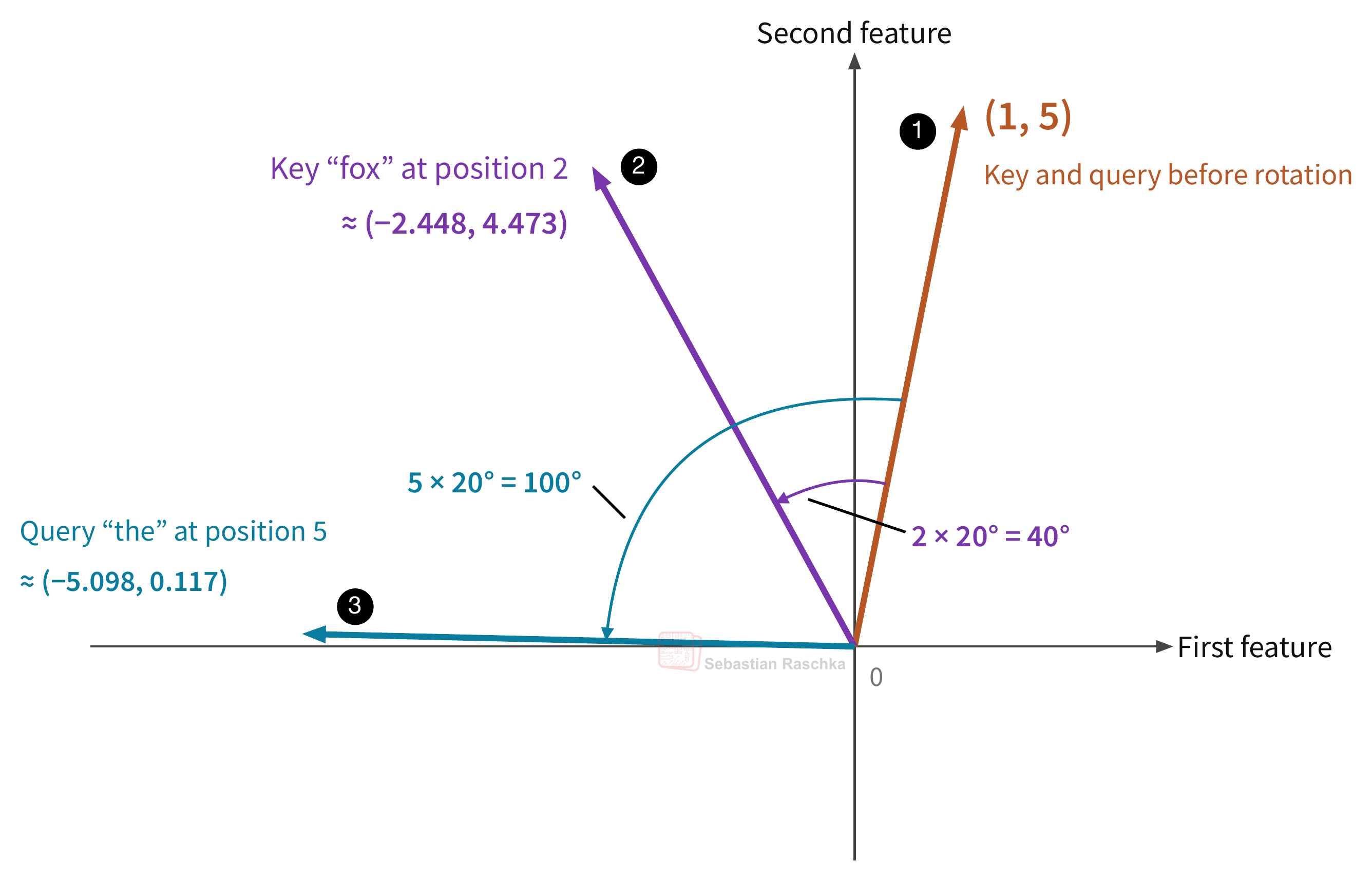Figure 18: Starting from (1, 5), RoPE rotates the key pair at position 2 by 40° and the query pair at position 5 by 100°.

To illustrate what’s happening in the figure above, for example, plugging cos 40° ≈ 0.766 and sin 40° ≈ 0.643 into the rotation from Figure 16 gives the new key coordinates:

Then, changing 40° to 100°, using the same equation as above, the rotated query pair becomes q′ ≈ (−5.098, 0.117). But the important point is that both arrows still have length √26. Only the rotation changes but the vectors keep the same lengths after the transformation.

So, for a query pair (a, b) at position m, the two operations here are.

For the key pair at position n, we use the same equations with nθ.

(Section 4 later shows how RoPE calculates the angular frequency for each feature pair.)

To close this section, for those more comfortable reading code, everything about RoPE illustrated so far can be written in code, as follows:

import torch

query_head = torch.tensor([1., 2., 3., 4., 5., 6., 7., 8.])
key_head = query_head.clone()

# Split-half pairing gives (1, 5), (2, 6), (3, 7), and (4, 8).
query_pairs = torch.stack(query_head.chunk(2), dim=-1)
key_pairs = torch.stack(key_head.chunk(2), dim=-1)

# Take the first feature pair from each head.
q = query_pairs[0]
k = key_pairs[0]

m = 5  # Query position (in our example, "the")
n = 2  # Key position (in our example, the first "fox")
theta = torch.deg2rad(torch.tensor(20.0))  # Radians per token position

def rotate_pair(pair, angle):
    a, b = pair
    c, s = torch.cos(angle), torch.sin(angle)
    return torch.stack((a * c - b * s, a * s + b * c))

k_rot = rotate_pair(k, n * theta)  # 2 × 20° = 40°
q_rot = rotate_pair(q, m * theta)  # 5 × 20° = 100°

print(f"Original key:   ({k[0]:g}, {k[1]:g})")
print(f"Original query: ({q[0]:g}, {q[1]:g})")
print(f"Rotated key:    ({k_rot[0]:.3f}, {k_rot[1]:.3f})")
print(f"Rotated query:  ({q_rot[0]:.3f}, {q_rot[1]:.3f})")

The resulting values are:

Original key:   (1, 5)
Original query: (1, 5)
Rotated key:    (-2.448, 4.473)
Rotated query:  (-5.098, 0.117)

If we rotate all 4 pairs in the 8-feature query (and key) vector(s), we get the vectors below. (We’ll come back to how we go from rotating one pair to rotating all of them later.)

Original key:   (1, 2, 3, 4, 5, 6, 7, 8)
Original query: (1, 2, 3, 4, 5, 6, 7, 8)
Rotated key:    (-2.448, 1.577, 2.951, 3.994, 4.473, 6.125, 7.021, 8.003)
Rotated query:  (-5.098, 0.928, 2.877, 3.986, 0.117, 6.256, 7.051, 8.007)

3.4 How the relative offset changes the attention score in RoPE

Note that, as shown above, the query and key heads have eight features each, which we previously grouped into 4 pairs with two elements each, like (1, 5), and (2, 6), and so on. For simplicity here we’ll follow just the first pair in each head, (1, 5), formed by taking the entries at indices 0 and 4:

Original key:   (1, 5)
Original query: (1, 5)
Rotated key:    (-2.448, 4.473)
Rotated query:  (-5.098, 0.117)

As shown above, in our example, those entries have values (1, 5) in both heads before the rotation.

Also, as in the code above, let’s use the notation q =(q1, q2) and k =(k1, k2) for these two pairs. To compute their dot product, using the standard dot product formula, we multiply corresponding coordinates and add the products:

Before rotation, the pairs have a dot product of 1 × 1 + 5 × 5 = 26. Using the rounded coordinates from the previous Figure 18 gives the contribution from the first pair after rotation:

We can see why by writing the dot product in terms of the lengths of the two vectors (arrows in Figure 18) and the angle ϕ between them.

In both cases, the vector length is √26. The query (position 5) is rotated by 100° and the key (position 2) is rotated by 40°. The vectors (arrows) start from the same direction, so they end up being 60° apart after rotation. Their exact dot product is 26 × cos(60°) = 13.

Now let’s see what happens if we move just the key from position 2 to position 3, but we keep its starting coordinates (1, 5) fixed. The key’s rotation changes now from 2 × 20° = 40° to 3 × 20° = 60°. The query still rotates by 100°, so the angle between the arrows shrinks to 40° and the dot product changes from 13 to 26 × cos(40°) ≈ 19.92. So, moving the key one position closer changed the dot product even though we started with the same feature values.

Why do these dot products matter? In attention, we sum the contributions from all feature pairs to get the query-key dot products. RoPE can change those dot products and thus the weights that softmax assigns to the value vectors.

In the attention equation above, Q′ and K′ are matrices that contain the rotated queries q′ and keys k′ for one head, V contains the values, and d is the head dimension.

3.5 Why shifting both positions preserves the attention score in RoPE

Now that we illustrated the computation of the dot products, which is at the core of the attention mechanism, let’s return to positions m = 5 and n = 2. If we shift both positions to the right by three positions, we get m = 8 and n = 5. Each rotation gains 60° (the query goes from 100° to 160°, and the key goes from 40° to 100°), however, the angle between the vectors stays the same. The dot product for this feature pair is still 13.

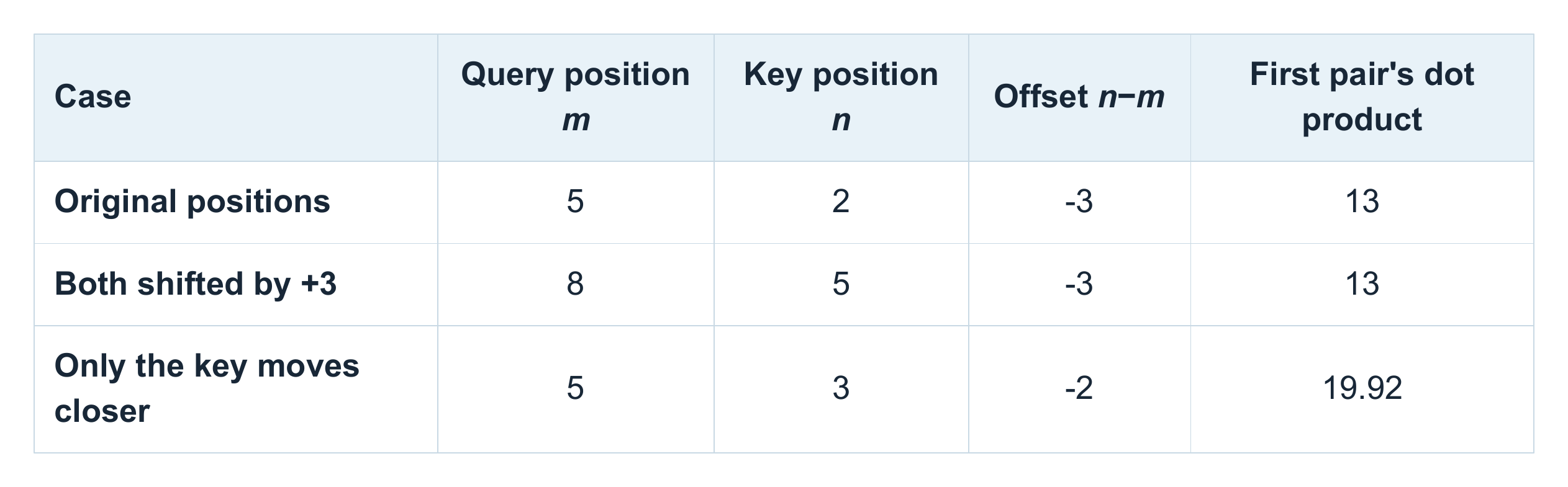Figure 19: The first pair’s dot product at three different position settings.

The key is that the difference between the rotation angles is

If we keep the original query and key vectors fixed and shift both token positions by the same amount, RoPE adds the same rotation to both vectors. The angle between them stays the same, so their dot product stays the same. Note that Figure 20 below uses smaller angles than the actual example (20° per position) to keep the picture readable.

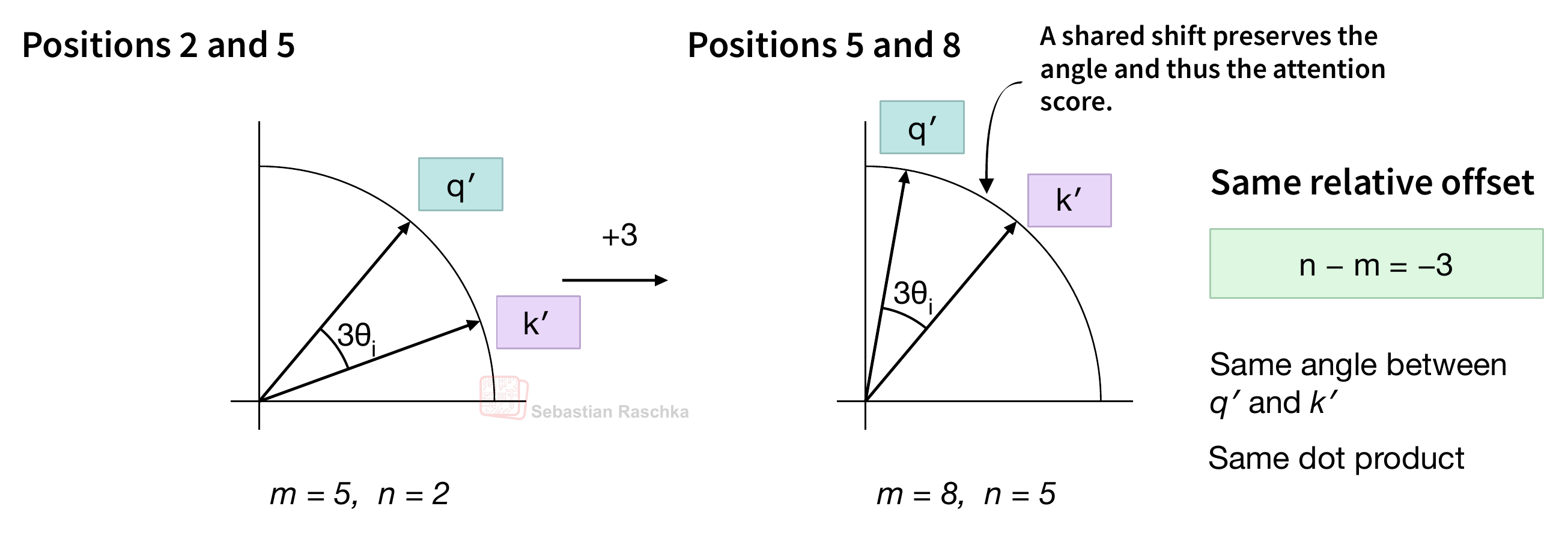Figure 20: A shared position shift preserves the relative angle and dot product for fixed query and key features.

The examples above and Figure 20 illustrate the main idea behind RoPE. We use each token’s position to rotate the corresponding query and key in the attention module. In the query-key dot product, what matters is how much one vector rotates relative to the other. For each feature pair, this difference in rotation depends only on the offset between the two tokens.

To illustrate this in the big picture context, in Figure 21, each row collects the scores for one query. If we consider row 5, the query for “the”, and column 2, the key for “fox”, the attention score between those two is computed as the dot product between the two rotated versions of the query and key vector.

Figure 21: The attention scores for one head before softmax. Gray cells mark future keys excluded by the causal mask.

What’s the point, again? Let’s once more consider “The red fox jumps over the gray fox.” If we add 100 tokens (e.g., think system prompt) before the sentence, the first “fox” and the second “the” move from positions 2 and 5 to 102 and 105. However, a prefix of any length shifts both positions equally, so they still stay exactly three positions apart. This means, each vector (arrow) gains the exact same additional rotation, which preserves the angle between them and their dot product (assuming we hold the unrotated query and key vectors fixed; in a real model, a new prefix of 100 tokens can change those vectors by changing what the tokens attend to).

Figure 22 tracks this comparison in the attention score matrix. The right panel shows the rows and columns for the sentence after we add the prefix. In our toy example, the first pair still contributes 13 to the dot product.

Figure 22: The highlighted score moves from row 5, column 2 to row 105, column 102. It keeps the same value if we hold the query and key vectors fixed before rotation.

As you may recall, in the original transformer’s sinusoidal encoding, a fixed offset also corresponds to a fixed rotation within each sine/cosine pair. But that shared rotation applies only to the position vectors (added to the input vector) instead of the key and query vectors inside the attention mechanism.

Figure 23 compares what this shift changes in the three methods we covered so far.

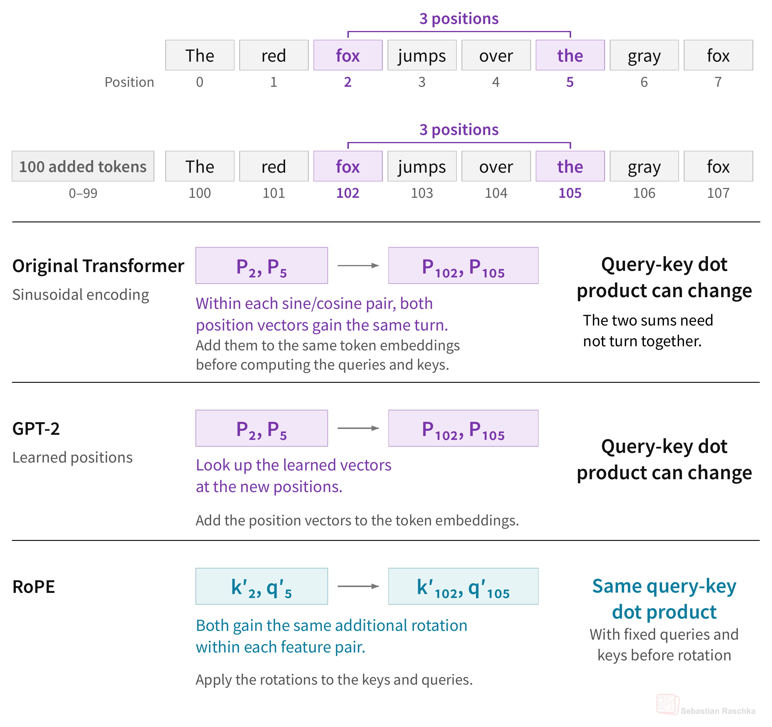Figure 23: The same position shift under sinusoidal encodings, GPT-2’s learned position embeddings, and RoPE.

3.6 Bonus: Combining the pairs into a complete head in RoPE

To see how the relative offset affects the dot product, we focused on one feature pair in the query and key. Now let’s put all four pairs together and see how RoPE rotates the full eight-feature vectors in one attention head. (Please feel free to skip this section if it is too much technical detail.)

Figure 24 picks up where Figure 17 left off. We rotate each of the four pairs, then put the results back in the query’s original feature order.

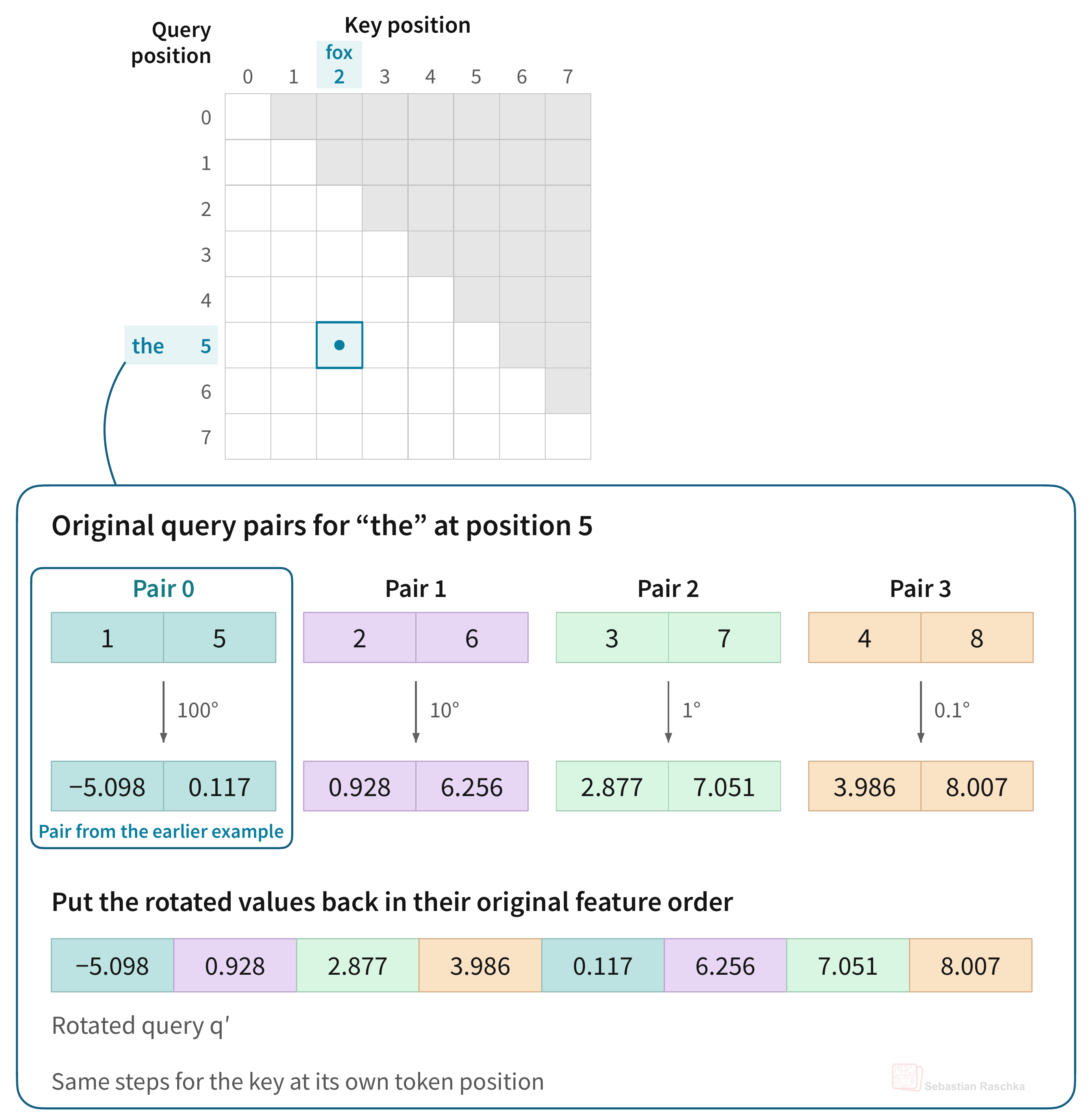Figure 24: RoPE rotates each pair of query features at its own angle. (The same can be applied to the key, which is not shown to keep the illustration simple).

Figure 24 above shows the rotated query q′(at the bottom). Similarly, we could get the rotated key k′ by repeating the same steps at the key’s position.

Recall the two equations from Section 3.3. For query pair i with input values (ai, bi), let ci = cos(mθi) and si = sin(mθi). These are the cosine and sine of the rotation angle for that pair at query position m:

Figure 25 below shows the same four rotations between the four pairs as a single matrix multiplication, q′ = Rmq.

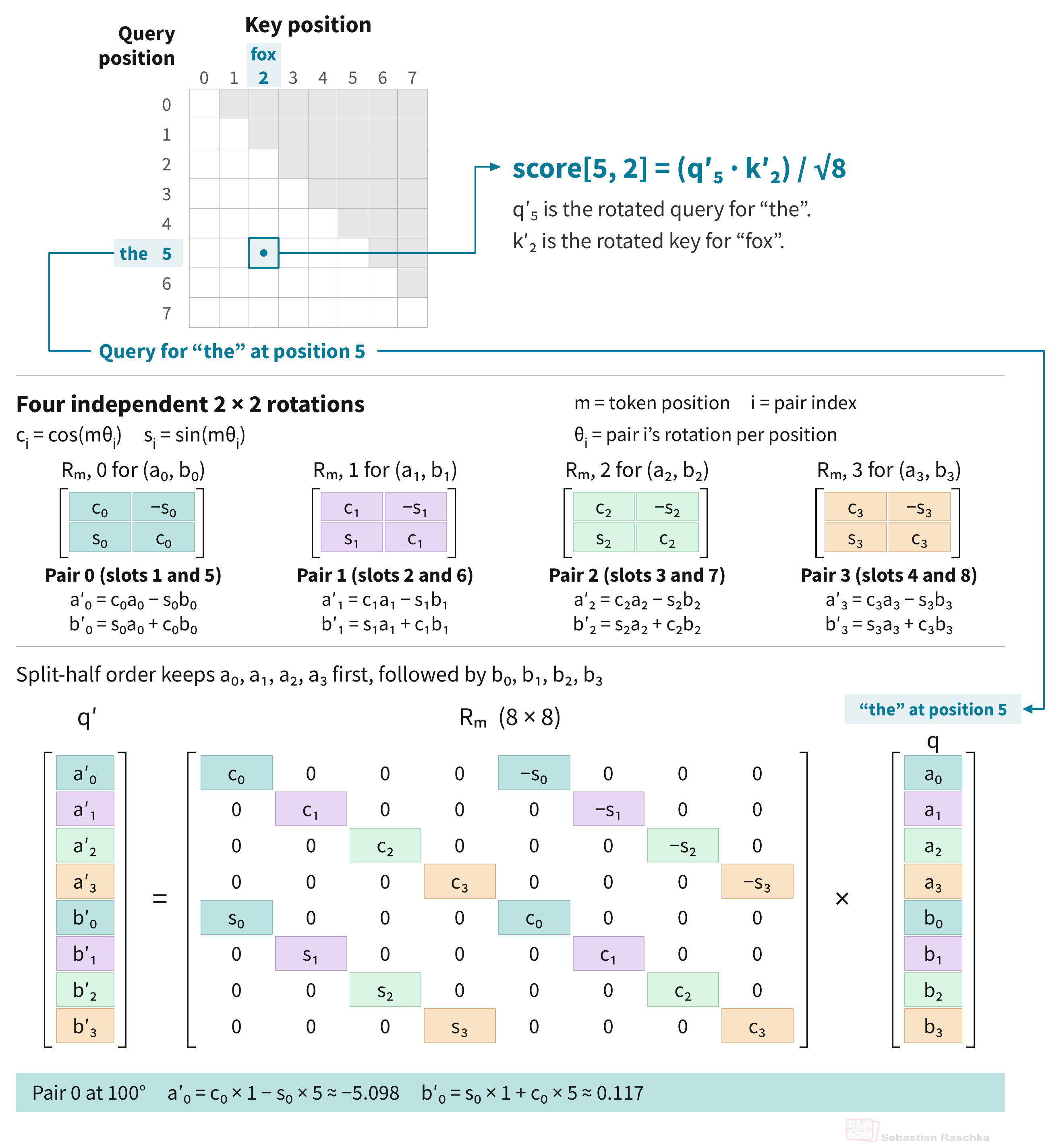Figure 25: The four rotations from Figure 24 written as one matrix multiplication. The pair labels show where each rotation goes in the full matrix.

4. Computing rotation frequencies in RoPE?

A full attention head uses multiple frequencies so that some feature pairs change more drastically (”quickly” in RoPE terms) with position and others change more gradually (”slowly” in RoPE terms). This serves the same purpose as the multiple frequencies in the original transformer’s sinusoidal encodings.

However, instead of us assigning these manually, for a head with d features, standard full RoPE computes one frequency for each of its d/2 pairs as follows:

Here,

• d is the head dimension (it has to be even so that all features can be arranged in pairs).
• b is a chosen base value (hyperparameter) that determines the spacing of the frequencies.
• θi is pair i‘s frequency in radians per token position.

The original RoFormer paper uses b = 10,000, borrowing the original transformer’s frequency formula with head dimension d in place of embedding width dmodel.

For example, with head dimension d = 8 and base b = 10,000, we get frequencies [1, 0.1, 0.01, 0.001] radians per position.

5. Bonus: Implementing RoPE in PyTorch

If you want to see RoPE in a complete model, I recommend checking out my end-to-end Qwen3 from-scratch implementation.

Since code can be an effective medium for explaining and understanding concepts, the following subsection will walk you through the core parts that we have covered so far, if you are interested. Otherwise, please feel free to fast forward to section 6, on Positional choices in modern architectures.

So, for the following code snippets, we’ll use the same split-half rotation convention as mentioned earlier (the interleaved convention will also be covered, no worries). First, we’ll apply it to one query vector, then we’ll use it on queries and keys inside the attention mechanism.

5.1 Computing and applying the rotations

First, let’s reuse the 8-feature query from Figure 24. For convenience, below are its four feature pairs before rotation.

Detail from Figure 24. The eight query features form four pairs in the split-half layout.

In the earlier non-coding example, we chose a frequency of 20° per token position for the first pair to keep the math simple. Here, we’ll use the original RoPE formula from the previous Section 4 above, θi = b−2i/d, with head dimension d = 8 and base b = 10,000.

Figure 26 shows how the two functions work together to apply these rotations.

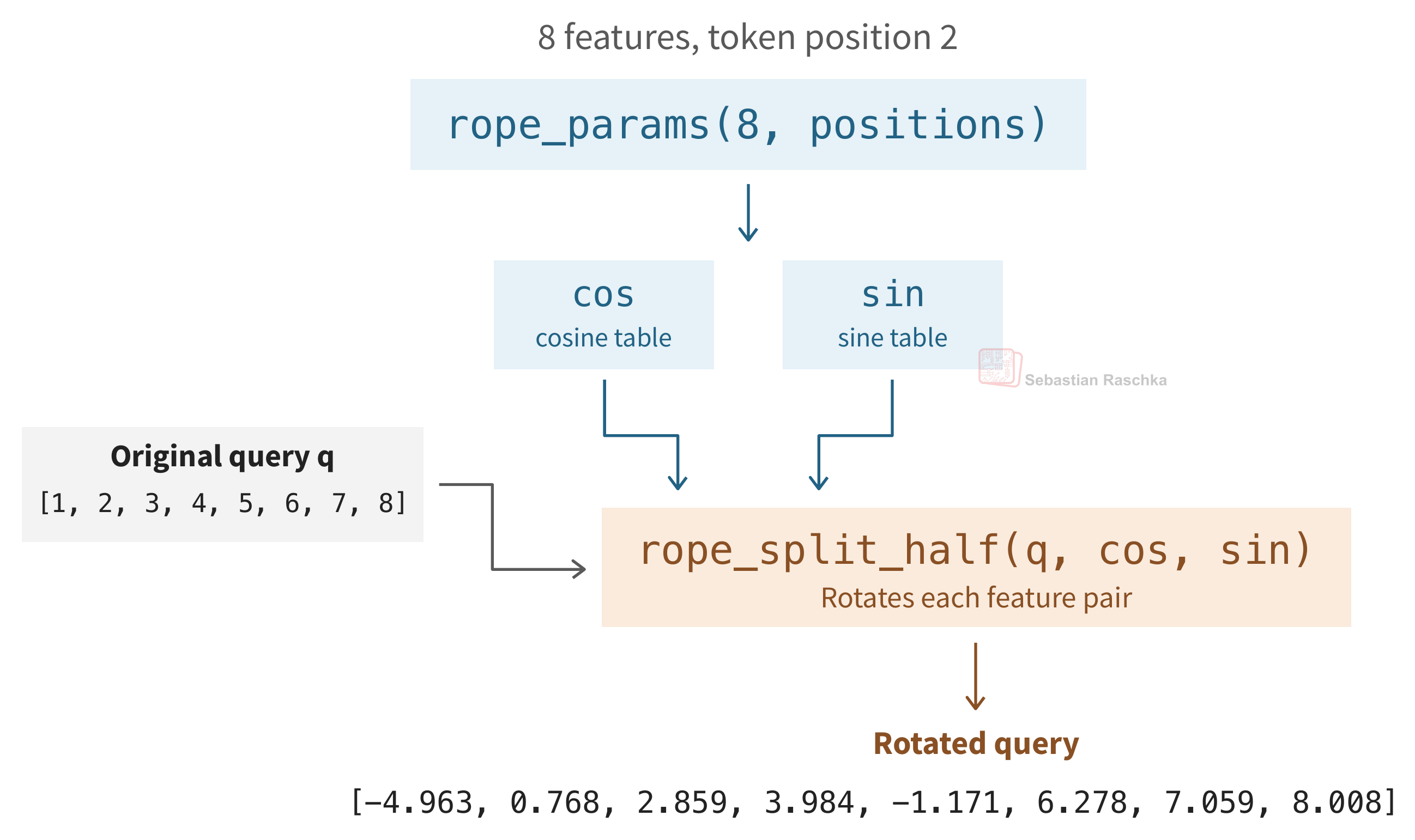Figure 26: rope_params returns the cosine and sine tables for token position 2. rope_split_half takes those tables and the original query and returns the rotated query.

As shown in the figure above, first, rope_params determines how far to rotate each pair, returning two “tables” that store the cosine and sine of those angles. Or, in other words, rope_params computes the cosine and sine of each rotation angle, which depends on the token’s position and the feature pair’s frequency.

import torch

def rope_params(head_dim, positions, base=10_000):
    assert head_dim % 2 == 0
    indices = torch.arange(0, head_dim, 2, device=positions.device)
    inv_freq = base ** (-indices.float() / head_dim)
    angles = positions.float()[:, None] * inv_freq[None, :]
    return angles.cos(), angles.sin()

The indices array in the rope_params function contains the 2i values from the frequency formula in Section 4:

For our eight-feature query, the indicesare [0, 2, 4, 6], that is, one 2i value for each feature pair. Suppose we use the common base b = 10,000. And following our earlier examples, we choose a small head dimension of d = 8. In this case, the inv_freq then computes the four pair frequencies θi = b−2i/d as follows:

As we can see above, the resulting inv_freq has one frequency θi for each of the four feature pairs ( measured in radians) per token position.

Next, the angles then multiplies each pair’s frequency θi with the token position m, which computes the rotation angle mθi. In our example, with positions = [2], we get:

Finally, rope_params takes the cosine and sine of each angle and outputs them as two so-called cosine and sine tables, cos and sin. In both tables, each row is a token position and each column is a feature pair. Since we only use token position 2 here, each table has shape (1, 4), with the single row shown below:

For the example in Figure 26, each table has one row for token position 2 and four columns, one for each feature pair. Figure 27 shows the rotation angle for each pair and the corresponding entries in the two tables.

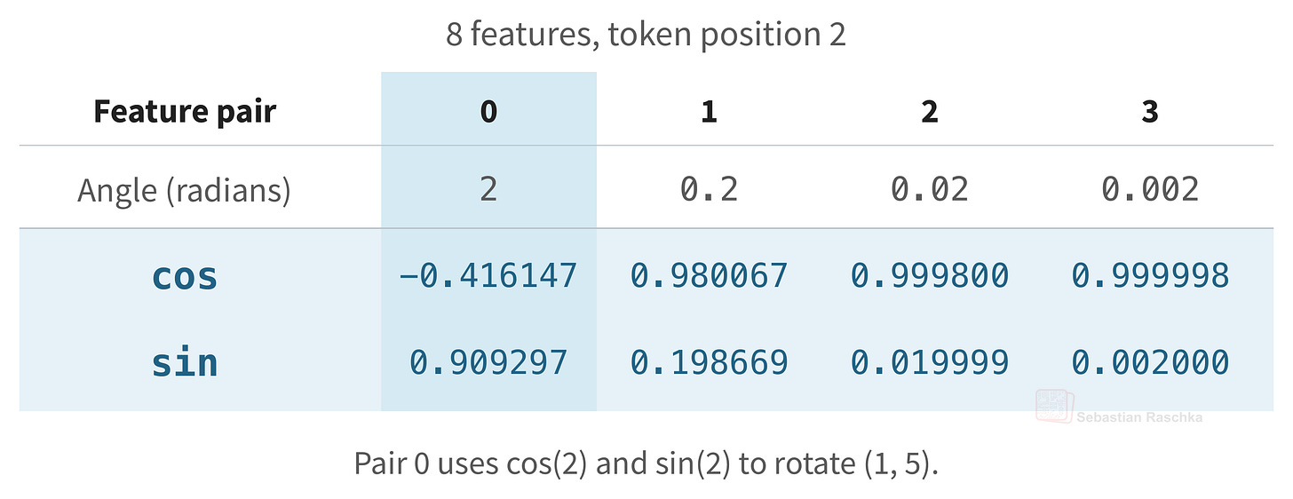
Figure 27: The two tables returned by rope_params for token position 2. The highlighted column gives the cosine and sine used to rotate the first feature pair, (1, 5).

In short, rope_params computes the cosine and sine of each rotation angle, which depends on the token’s position and the feature pair’s frequency.

In a real-world scenario, if we pass rope_params 1,024 token positions for a context size of 1024, and a head dimension of 128, it returns two tensors, cos and sin, each with shape (1024, 64) since a head with 128 features has 64 pairs.

The tables have no batch or head dimension, and we broadcast each (1024, 64) table across the batch and head dimensions. So, if we have multi-head attention or grouped query attention with 32 heads, feature pair 0 at token position 2 uses the same rotation angle in all 32 heads. Each head rotates its own feature values, so the rotated queries can still differ across heads. Also, the same entries can be reused across queries, keys, and heads that use the same positions and frequencies. In short, we only need to (pre)compute these tables once per model for all positions up to a maximum supported context size.

Technically, it would also be possible to store these tables alongside the model weights; but they are so incredibly cheap to compute that storing them on disk would be overkill.

Next, rope_split_half uses those cosines and sines to rotate the actual features in the query and key vectors inside attention.

def rope_split_half(x, cos, sin):
    first, second = x.float().chunk(2, dim=-1)
    return torch.cat((
        first * cos - second * sin,
        first * sin + second * cos,
    ), dim=-1).to(x.dtype)

Considering the simple 8-feature example once more, the .chunk in the code snippet above splits the query into [1, 2, 3, 4] and [5, 6, 7, 8] and lines up the two entries in each pair. For example, the first slot of each half gives us (1, 5), the second (2, 6), and so on. The two expressions inside torch.cat compute the rotated halves using the equations from Section 3.3:

Note that here, everything denoted with ai corresponds to the first half of the query, and everything denoted with bi comes from the second half. The first expression inside torch.cat computes all the *ai′*values, and the second computes all the bi′ values.

Then, we concatenate the halves, which puts each value back in its original index position via torch.cat.

Here’s the code that produces the rotated query in the earlier Figure 26. The shown reshape (1, 1, 1, 8) just brings the simple toy array into the expected format: one batch item, one head, one token, and eight features.

positions = torch.tensor([2])
cos, sin = rope_params(8, positions)

q = torch.arange(1., 9.).reshape(1, 1, 1, 8)
q_rot = rope_split_half(q, cos, sin)
print(q_rot[0, 0, 0])

With several positions, each token simply picks up its own row from the cos and sin tables. Through broadcasting, PyTorch reuses these same tables across all batch items and attention heads.

5.2 Using RoPE inside causal attention

So far, we coded the RoPE utility functions. Let’s now use it in the real context, the attention mechanism. Here, we use the standard frequency schedule for two 8-feature heads and four token positions. We use random query, key, and value tensors to keep the example self-contained, but as mentioned before, you can optionally also check the end-to-end Qwen3 from-scratch implementation with real query, key, and values produced by the pre-trained model.

torch.manual_seed(123)

q = torch.randn(1, 2, 4, 8) # 1 batch, 2 heads, 4 tokens, 8 head dim
k = torch.randn(1, 2, 4, 8)
v = torch.randn(1, 2, 4, 8)
positions = torch.arange(4)

cos, sin = rope_params(8, positions)
q_rot = rope_split_half(q, cos, sin)
k_rot = rope_split_half(k, cos, sin)
scores = q_rot @ k_rot.transpose(-2, -1) / q.shape[-1] ** 0.5

future_mask = positions[None, :] > positions[:, None]
masked_scores = scores.masked_fill(future_mask, -torch.inf)
weights = torch.softmax(masked_scores, dim=-1)
context = weights @ v

Note that only q and k but not v pass through RoPE. The resulting raw attention scores are stored in a tensor of shape (1, 2, 4, 4), that is, one row for each query position, and a column for each key position, and 4x4 since we have four tokens where each attends to each other.

Then, using a conventional attention code implementation, the causal mask replaces the scores for future keys with negative infinity, so they get zeroed after the softmax. The resulting context tensor has shape (1, 2, 4, 8); the 4 because we have four tokens, and the 8 because the embedding dimension was originally 8.

We can also check that our claim about relative offsets holds, meaning that adding 3 to each position should change the position but preserve the query-key offsets:

cos_shifted, sin_shifted = rope_params(8, positions + 3)
q_shifted = rope_split_half(q, cos_shifted, sin_shifted)
k_shifted = rope_split_half(k, cos_shifted, sin_shifted)
scores_shifted = (
    q_shifted @ k_shifted.transpose(-2, -1) / q.shape[-1] ** 0.5
)
torch.testing.assert_close(scores, scores_shifted) 
# Should return True

5.3 An alternative feature-pairing convention

I mentioned the split-halves convention many times throughout this article. The original RoPE paper uses the alternative interleaved convention, as does the original LLaMA implementation (but as mentioned before, most code implementations now use the split-halves, because it makes it easier, in code, to rotate all pairs at once with element-wise sine and cosine operations.)

To illustrate the difference between the two layouts, Figure 28 below uses the same 8-feature vector in both rows.

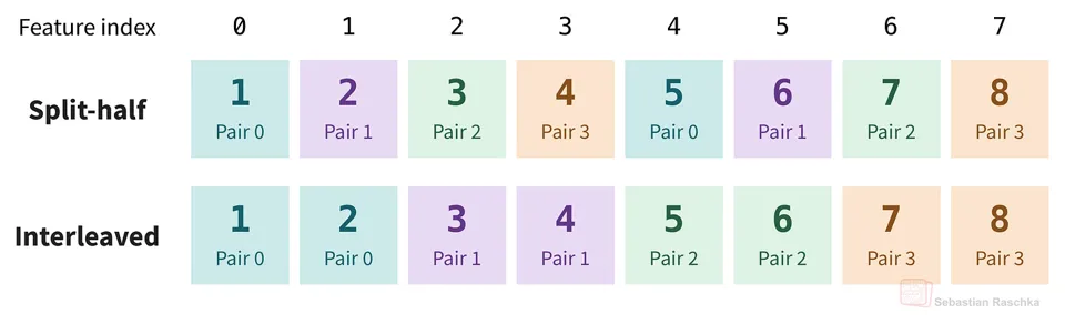
Figure 28: Split-half pairs each feature in the first half with the corresponding feature in the second half. Interleaved pairs adjacent features.

The interleaved implementation uses the same two equations, but selects alternating features and interleaves the outputs.

def rope_interleaved(x, cos, sin):
    even, odd = x.float()[..., 0::2], x.float()[..., 1::2]
    return torch.stack((
        even * cos - odd * sin,
        even * sin + odd * cos,
    ), dim=-1).flatten(-2).to(x.dtype)

But mathematically, the layouts are equivalent when we account for the feature order. So, rearranging the entries [1, 2, 3, 4, 5, 6, 7, 8] to [1, 5, 2, 6, 3, 7, 4, 8] makes the split-half pairs adjacent with pairs (1, 5), (2, 6), and so on. If we apply the same rearrangement to both queries and keys, it results in identical dot products.

order = torch.tensor([0, 4, 1, 5, 2, 6, 3, 7], device=q.device)
q_rot_interleaved = rope_interleaved(q[..., order], cos, sin)
k_rot_interleaved = rope_interleaved(k[..., order], cos, sin)
scores_interleaved = (
    q_rot_interleaved @ k_rot_interleaved.transpose(-2, -1)
    / q.shape[-1] ** 0.5
)

torch.testing.assert_close(q_rot[..., order], q_rot_interleaved)
torch.testing.assert_close(k_rot[..., order], k_rot_interleaved)
torch.testing.assert_close(scores, scores_interleaved)
# This should all return True

The outputs retain the reordered features, so we compare them with the split-half outputs in that same order. Applying the two layouts to the original vector however would give different scores.

6. Positional choices in modern architectures

RoPE has been a staple in most (open-weight) LLMs since the original LLaMA model. Of course, proprietary models may use it as well, but it’s always hard to say anything with 100% certainty about proprietary models.

However, in recent years, many architectures have been moving away from full-blown RoPE in every transformer block. In the following subsection, we will discuss some of these variants.

For instance the full RoPE implementation we discussed and implemented in the sections above rotates every feature pair in every query and key head.

In the following examples in the subsections above below, we will see that models only rotate some features within a head, other models skip RoPE in some transformer blocks, and some models use a different approach and add position information directly to their attention scores.

6.1 Partial RoPE

As discussed throughout the article, regular “full” RoPE rotates all dimensions in each query and key head. Partial RoPE is a variant that rotates only a subset, while leaving the remaining dimensions unchanged.

For example, MiniMax-M3’s configuration uses 64 rotary dimensions within each 128-dimensional head. That gives 32 rotated feature pairs and 64 unchanged dimensions. The figure below illustrates how that looks like.

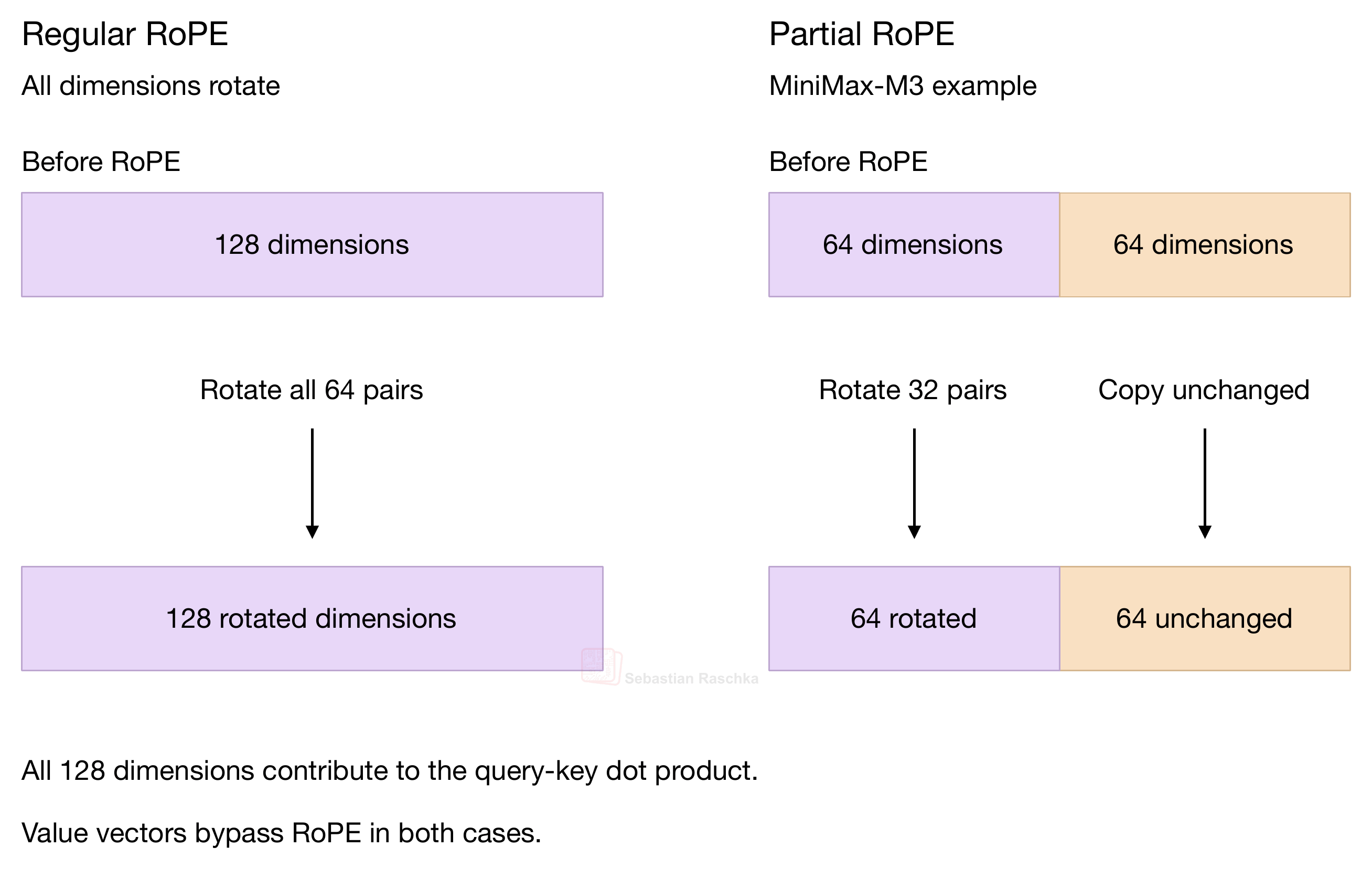Figure 29: Full RoPE and partial RoPE in a 128-dimensional head.

Note that if we look past the first transformer block, the unrotated features can still contain position information inherited from earlier transformer blocks.

Anyways, what’s the point behind partial RoPE? It saves some memory. For example, in the MiniMax-M3 example above, rotating half the features reduces the size of the precomputed cosine and sine tables also in half. So, with partial RoPE, instead of 64 columns, now each table only needs 32 columns. However, note that the KV cache still stores the full key and value vectors for each cached token.

For MiniMax-M3’s 1M-token context, rotating 64 of the 128 features halves the size of the precomputed cosine and sine tables, saving 0.134 GB (128 MiB) if the tables are stored in BF16. If the tables themselves were stored in NVFP4, the savings would be 0.038 GB (36 MiB), including the block scales.

Note that in experiments with 1B to 8B models, the Fractional Rotation, Full Potential? paper found that rotating around 10% of each head’s features often gave similar training loss and benchmark accuracy to full RoPE. However, full RoPE did better on some evaluations.

So, in my opinion, partial RoPE is hardly worth it.

6.2 NoPE layers

NoPE was coined in the The Impact of Positional Encoding on Length Generalization in Transformers paper and means no explicit positional encoding. The idea or observation is that an attention layer without any explicit position method still has a causal mask, where a query can attend only to itself and earlier tokens. And this causal masking implicitly provides positional information.

Let’s use the first four tokens from our earlier example, The red fox jumps. In Figure 30, the query for fox at position 2 can attend to The, red, and itself. The query for red at position 1 can attend to The and itself.

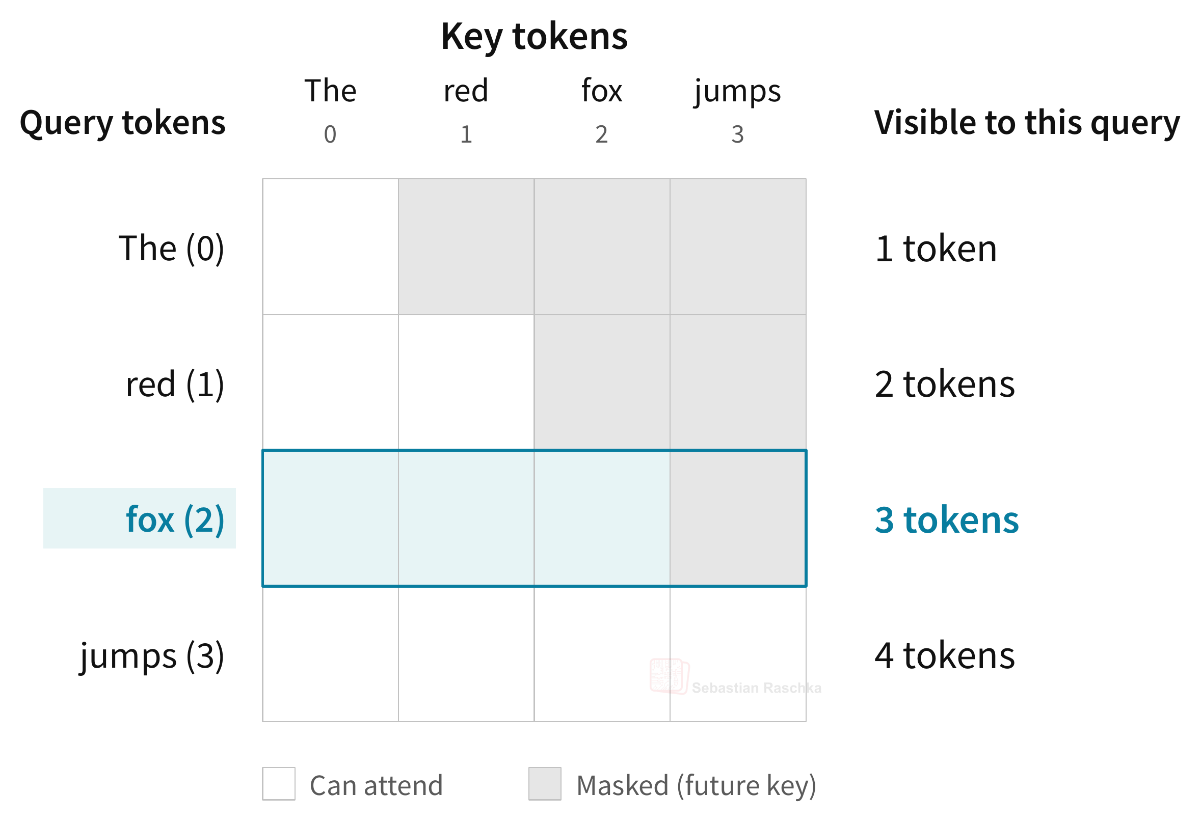Figure 30: Example of a causal mask in the attention mechanism.

So, the next question is how can the model use the causal mask as a position signal? Here’s a toy example adapted from the paper.

Suppose one feature of the value vectors is 1 for The and 0 for the other three tokens. Since the input only contains only one The, every visible prefix contains exactly one 1. If all non-masked keys get the same attention score, the softmax assigns every visible token equal weight.

So at fox, attention averages 1, 0, and 0, which gives 1/3. At jumps, it averages four values and gets 1/4. In other words, this output feature equals one over the prefix length, which a later layer can use as a signal for position.

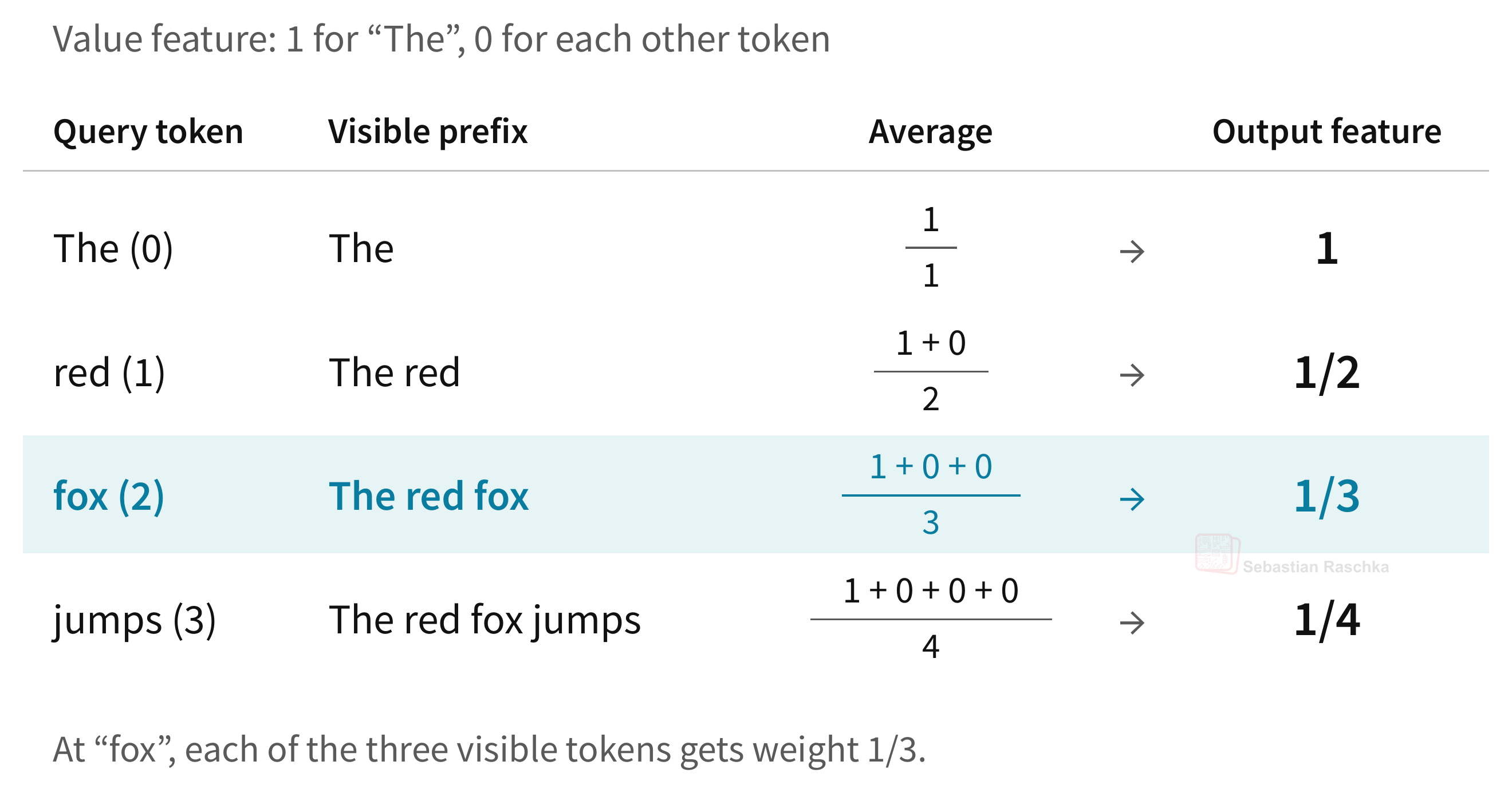Figure 31: With uniform attention, the contribution from The shrinks as the prefix grows. The query for fox assigns The a weight of 1/3.

Does NoPE work in practice? The researchers of the NoPE paper trained a tiny 107M-parameter decoder-only transformers from scratch on tasks such as copying, sorting, and addition to do some ablation.

When they tested the small model on examples longer than those seen during training, interestingly, NoPE ranked first overall across the ten tasks and ahead of RoPE. The researchers behind the NoPE paper also conducted a separate experiment with a larger 1.3B-parameter models trained on code. Here, NoPE also handled contexts beyond the training length, however, its next-token predictions got worse at the longest lengths tested.

Some of today’s open-weight LLMs even go so far and use NoPE in all layers. However, nowadays, it’s more common for models to omit RoPE in at least some layers, where layer here means transformer block.

To give a concrete example, SmolLM3 (3B parameters) applies RoPE in three layers and skips it in the fourth, repeating that pattern through 36 layers. Interestingly, the SmolLM3 authors mentioned that this layer pattern improved long-context performance.

(Also note that any later layer, following the first one, even though it may skip the rotation, still receives the inputs from preceding transformer blocks, so its queries and keys still receive some sort of position information from earlier layers.)

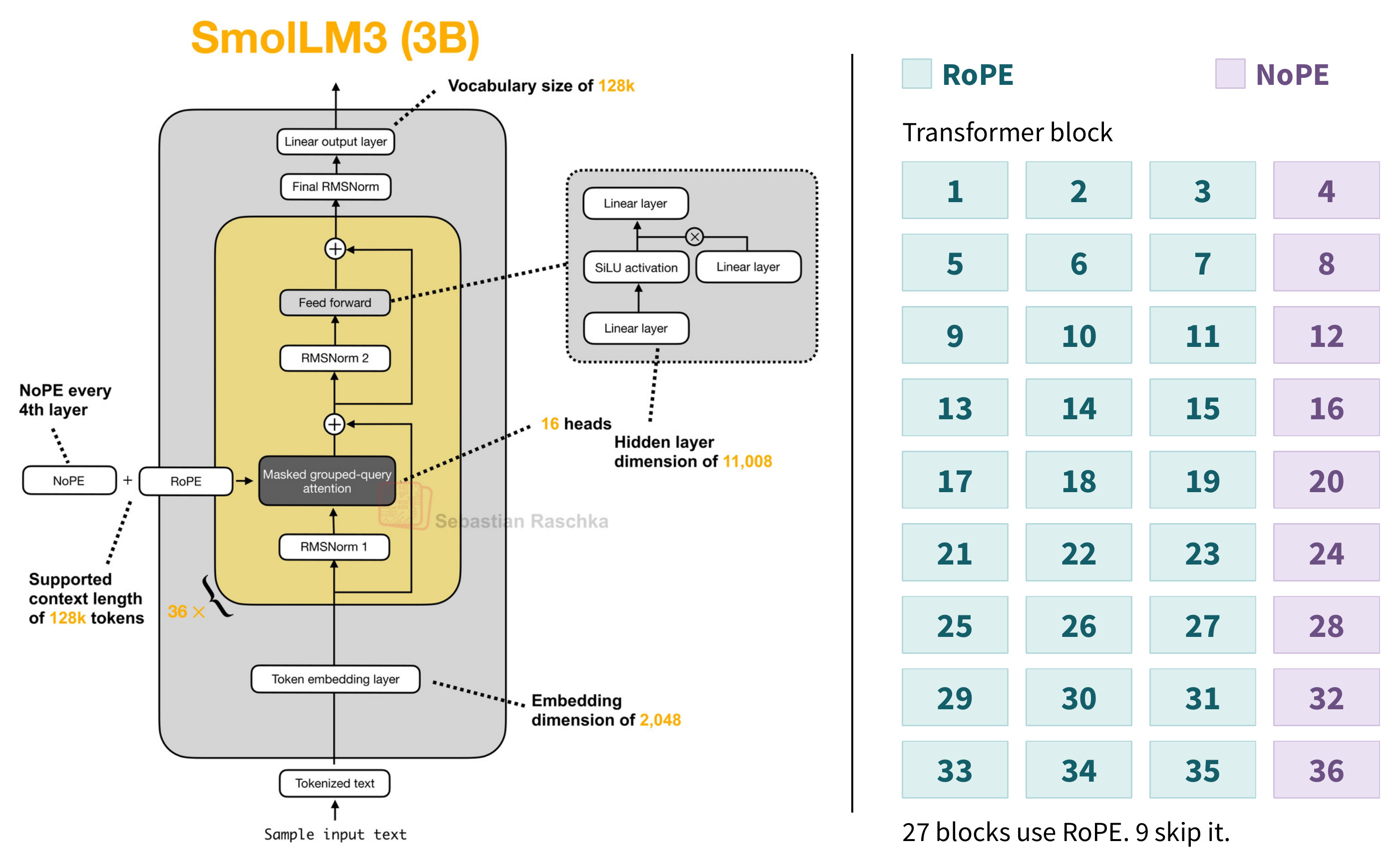Figure 32: SmolLM3’s architecture (left) and the positional method used in each of its 36 transformer blocks (right). Every fourth block skips RoPE. Architecture diagram from my LLM Architecture Gallery.

6.3 Learned relative position bias

Before we get to the overview and look at what modern architectures use, there’s one more method to introduce. For instance, Thinky’s Inkling uses a learned relative position bias in both its sliding-window and global attention layers. It computes the usual scaled dot product between a query and key, and then it adds a certain number to that score before the softmax in the attention score computation. That number depends on the query token’s hidden state and how many positions back the key is.

Let’s reuse our example sentence, “The red fox jumps over the gray fox.” (It’s the last time, I promise!) In the figure below, the “the” at position 5 is the query and “fox” at position 2 is the key. Inkling then uses the three-position gap between query and key and the hidden state for “the” to compute the bias, then adds it to the scaled dot product.

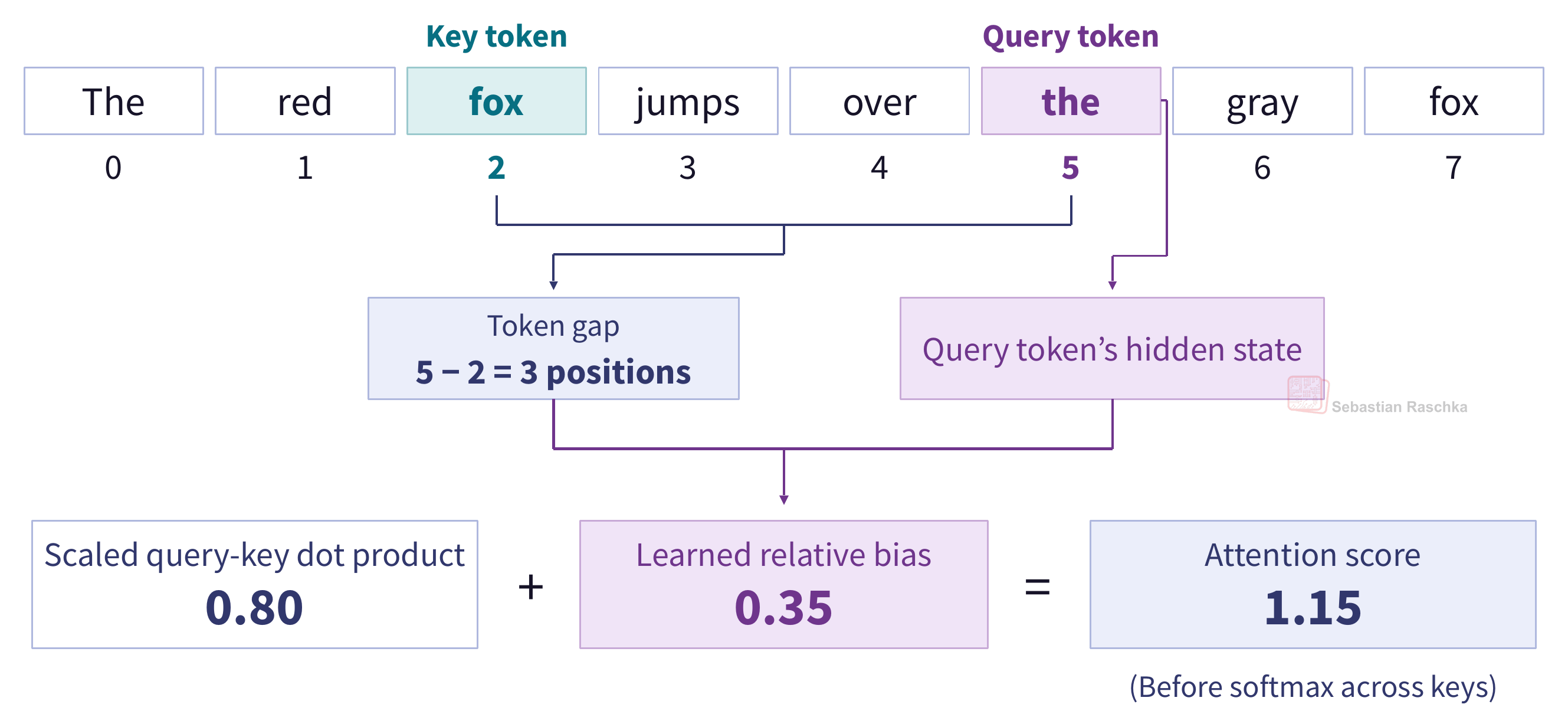Figure 33: Inkling adds a learned relative position bias to the scaled query-key dot product before softmax. The numbers are illustrative.

This is not an entirely new idea. Some of you may recall Google’s popular T5 (Text-to-Text Transfer Transformer) in 2019, which used a simpler version of this idea.

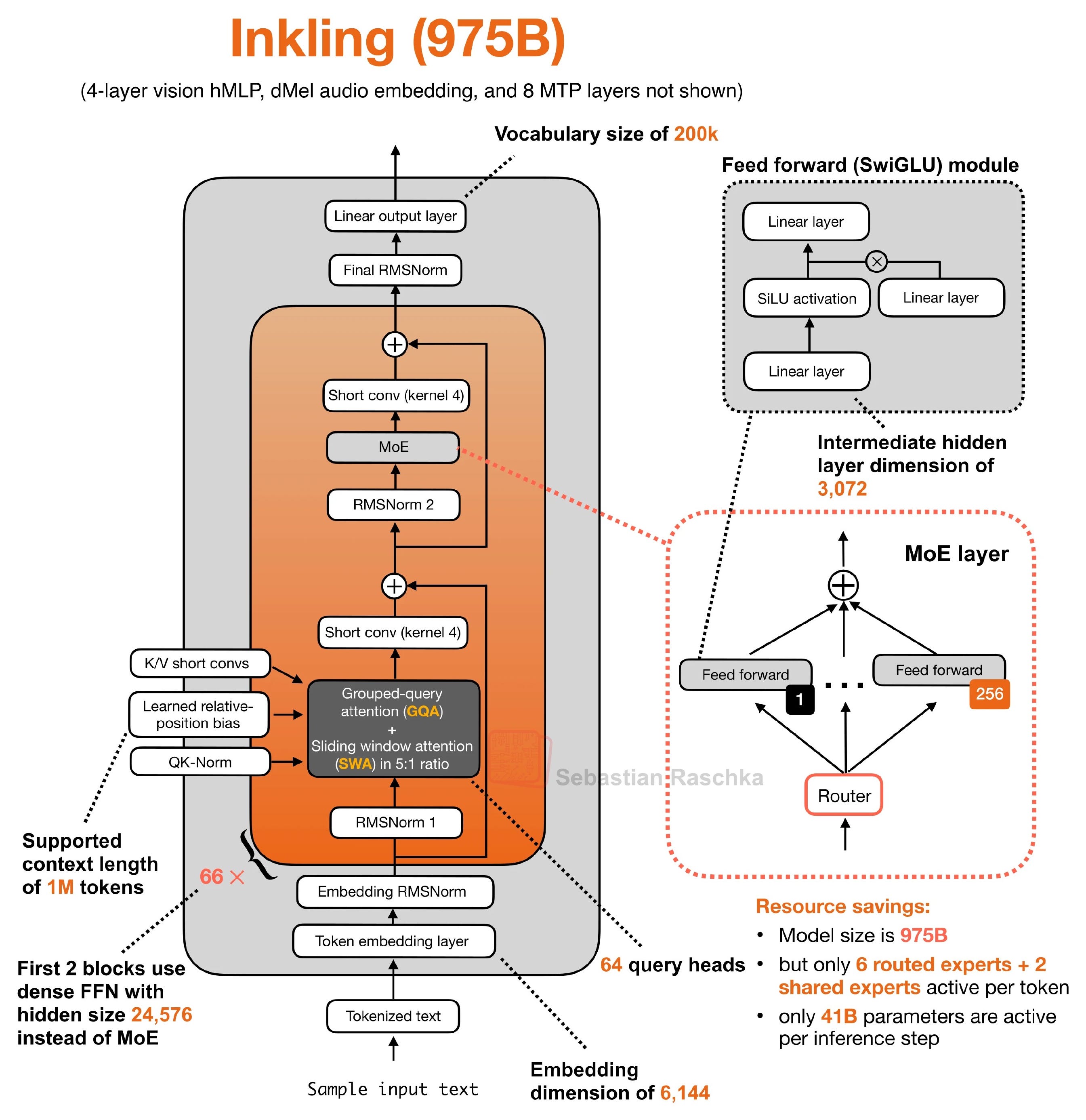Figure 34: The original Inkling (975B) architecture. The learned relative position bias feeds into the attention module. LLM Architecture Gallery

6.4 How these choices appear in recent models

Now, after all this build up, the interesting question is: which architecture uses which method? And what are the recent trends?

To answer this, I grouped the entries in my LLM Architecture Gallery by their listed release dates and compared the 2025 releases with the earlier and later releases in the 2026 snapshot. Each gallery card counts once, so multiple variants of an architecture can contribute to the results. LLM Architecture Gallery

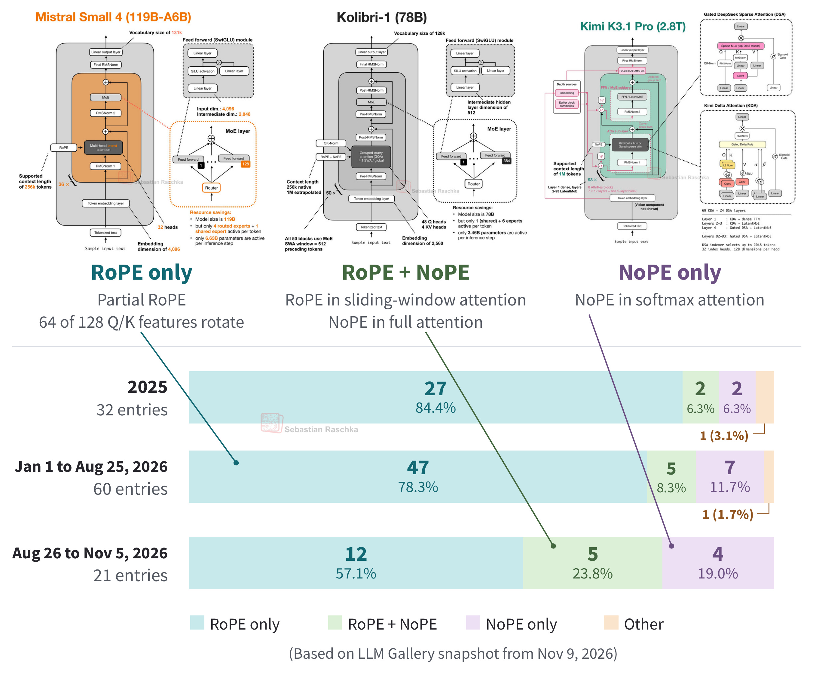Figure 35: The architecture diagrams illustrate which attention layers use RoPE, and the bars show the share of gallery entries in each category. Diagrams from my LLM Architecture Gallery.

As we can see in Figure 35 above, using RoPE in every softmax attention layer is still the most common choice. However, its use fell from 2025 to 2026, and then also in the latter half of 2026, which could be a trend.

Consequently, there is a growing number of models that mix RoPE and NoPE. The groups are still small, so it’s hard to say whether these trends will continue.

The NoPE only entries were all recurrent hybrids with softmax attention layers that use no explicit positional encoding. The “Other” category here refers to xLSTM 7B (2025) and Inkling (2026). xLSTM has no softmax attention layers. Inkling adds a learned bias to the attention scores before softmax, as we saw in Section 6.3.

Among the models that use RoPE, partial RoPE became more common from 2025 to 2026. It went from a minority of the RoPE models in 2025 to a majority in both 2026 groups, as shown in Figure 36.

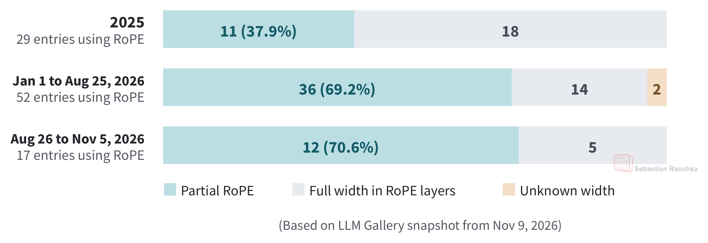Figure 36: Among gallery entries that use RoPE, partial RoPE rotates a subset of query and key features in at least one attention layer. Full-width entries rotate all query and key features in every layer that uses RoPE.

If you’d like to look up an individual model from the 2026 groups, Figure 37 below shows the 2026 gallery overview with the individual architectures labeled by position type. You can also browse the gallery interactively here.

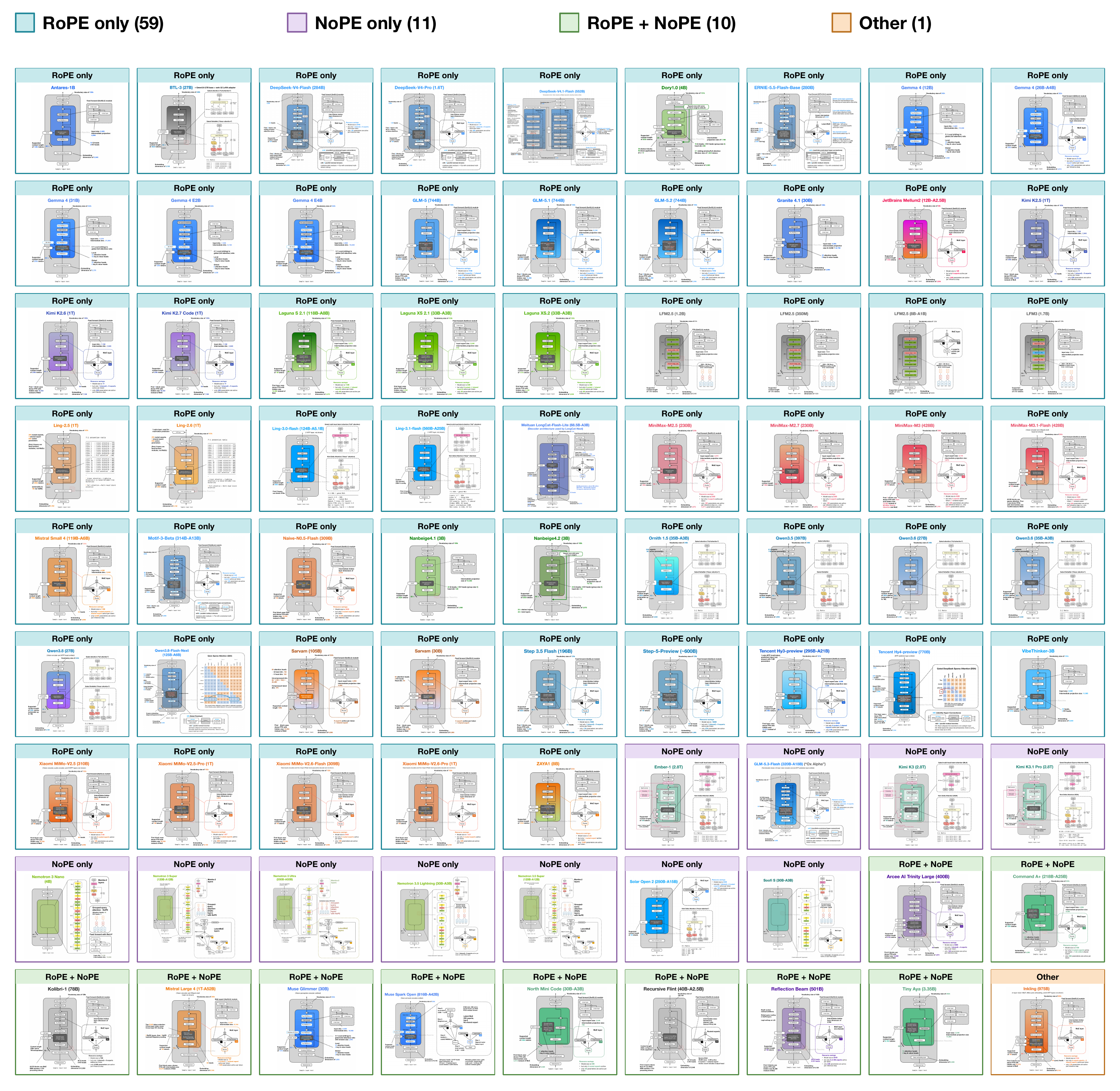Figure 37: The individual 2026 gallery entries behind the two 2026 bars in Figure 35.

7. Final thoughts

So, to recap, we discussed GPT-2 and the original transformer that add a position vector to each token embedding before the first transformer block. Then, modern LLMs switched to RoPE, which encodes relative position inside attention by rotating queries and keys. Surprisingly, RoPE remains as the most popular positional embedding method today.

Recently, however, Inkling picked up an idea from T5 to add a learned relative position bias to the attention scores before softmax. And then we also have NoPE-RoPE architectures, which omit RoPE in some layers.

It may be boring news, but as mentioned before, RoPE is still the predominant position embedding method, and I think this will carry over into 2027 for sure. Perhaps, though, we’ll see more architectures with an Inkling-like design coming up in 2027.

While this may sound “boring”, I am glad that I finally got this article on RoPE (and other position info methods) out, after so many years, so that I can add it to my collection of LLM “fundamentals” explainers.

If you are interested in the other architecture building blocks of LLMs, I still highly recommend starting with a GPT-2-style model, which will give you a solid understanding of the building blocks with the least amount of friction. And from there, you can then layer on additional methods (such as RoPE).

If you’d like to build that GPT-2-style model yourself, my first Build a Large Language Model (From Scratch) book walks through all the building blocks depicted in the figure below.

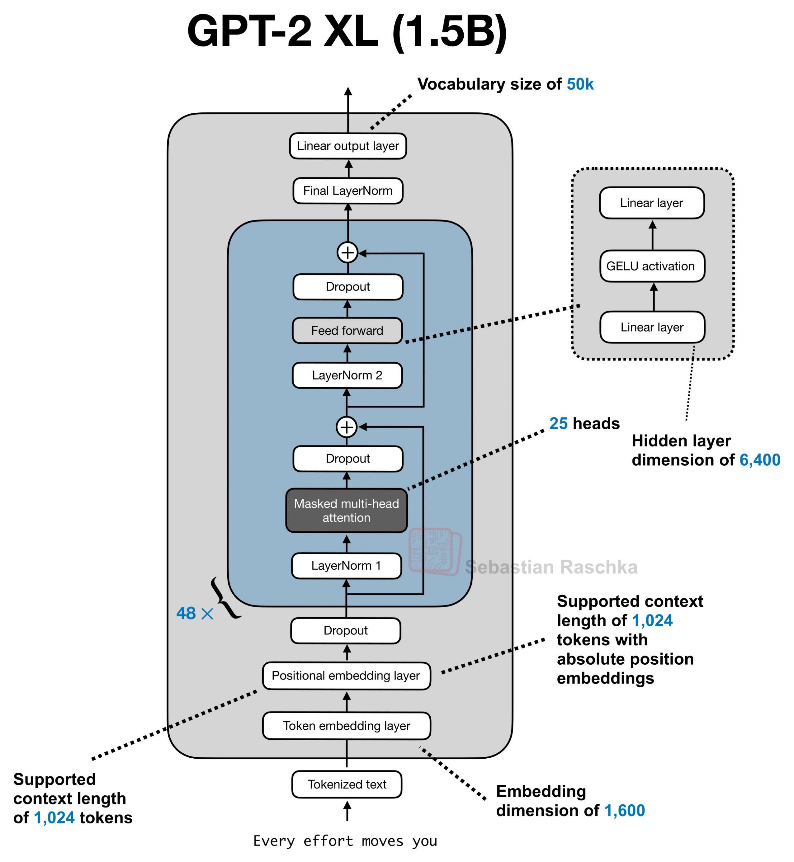Figure 38: GPT-2 XL provides a baseline for seeing what newer architectures change. LLM Architecture Gallery

For the methods that branch off from the GPT-2 baseline, I’ve collected some of my relevant blog articles below, starting with a refresher on self-attention: