Perceiver IO 集成至 Transformers:支持多模态统一建模
Hugging Face 将 Perceiver IO 模型正式集成至 Transformers 库,该架构通过潜在瓶颈机制实现了对文本、图像、音频及视频等任意模态数据的统一处理。作为首个完全基于注意力机制且具备高可扩展性的多模态模型,它打破了传统 Transformer 在输入长度和模态类型上的限制,并提供了光学流预测与图像分类等实际用例。
报道正文
本文目录12 个章节
Perceiver IO:一种可扩展、全注意力机制的模型,适用于任意模态
发布于 2021 年 12 月 15 日 在 GitHub 上更新 点赞 17
TLDR
我们已在 Transformers 中添加了 Perceiver IO,这是首个基于 Transformer 架构、能够处理各种模态(文本、图像、音频、视频、点云等)及其组合的神经网络。请查看以下 Spaces 以了解示例:
我们还提供了 多个 notebook。
下文将对该模型进行技术详解。
引言
由 Vaswani 等人于 2017 年最初提出的 Transformer,在 AI 社区引发了一场革命,起初显著提升了机器翻译领域的最先进(SOTA)水平。2018 年,BERT 发布,这是一种仅包含编码器的 Transformer 模型,它刷新了自然语言处理(NLP)的各项 benchmark,其中最著名的是 GLUE benchmark。
不久之后,AI 研究人员开始将 BERT 的理念应用到其他领域。举几个例子:
- Facebook AI 推出的 Wav2Vec2 证明了该架构可以扩展到音频领域
- Google AI 推出的 Vision Transformer (ViT) 展示了该架构在视觉任务上的卓越表现
- 最近,同样由 Google AI 推出的 Video Vision transformer (ViViT) 将该架构应用到了视频领域。
在所有这些领域中,得益于这一强大架构与大规模预训练的结合,最先进(SOTA)结果得到了显著提升。
然而,Transformer 架构存在一个重要的局限性:由于其 自注意力机制,它在计算量和内存占用方面的扩展性非常差。在每一层中,所有输入都被用来生成查询(queries)和键(keys),并计算成对的点积。因此,如果不进行某种形式的预处理,就无法将自注意力机制应用于高维数据。例如,Wav2Vec2 通过采用特征编码器来解决这一问题,将原始波形转换为基于时间的特征序列。Vision Transformer (ViT) 将图像分割为一系列不重叠的补丁(patches),这些补丁充当“token”。Video Vision Transformer (ViViT) 从视频中提取不重叠的时空“管状体”(tubes),这些管状体也充当“token”。为了让 Transformer 适用于特定模态,通常需要将数据离散化为 token 序列。
Perceiver
Perceiver 旨在通过在潜在变量集合上而非直接在输入上使用自注意力机制来解决这一局限性。inputs(可以是文本、图像、音频或视频)仅用于与潜在变量执行交叉注意力(cross-attention)。这种设计的优势在于,大部分计算发生在潜在空间中,而该空间的计算成本较低(通常使用 256 或 512 个潜在变量)。由此产生的架构对输入大小没有二次方依赖关系:Transformer 编码器仅线性依赖于输入大小,而潜在注意力则独立于输入大小。在一篇后续论文 Perceiver IO 中,作者进一步扩展了这一思想,使 Perceiver 也能处理任意输出。其思路类似:输出仅用于与潜在变量执行交叉注意力。请注意,在本博客文章中,我将互换使用“Perceiver”和“Perceiver IO”这两个术语来指代 Perceiver IO 模型。
HuggingFace Transformers 中的所有 Perceiver 变体均基于 PerceiverModel 类。要初始化一个 PerceiverModel,可以向模型提供以下 3 个额外实例:
- 预处理器(preprocessor)
- 解码器(decoder)
- 后处理器(postprocessor)
请注意,这些组件均为可选。只有当用户尚未自行对 inputs(如文本、图像、音频、视频)进行嵌入处理时,才需要 preprocessor。只有当需要将 Perceiver 编码器的输出(即 latent 变量的最后隐藏状态)解码为更有用的形式(例如分类 logits 或光流)时,才需要 decoder。只有当需要将 decoder 的输出转换为特定特征时,才需要 postprocessor(这仅在进行自编码任务时才需要,下文将详细说明)。架构概览如下图所示。
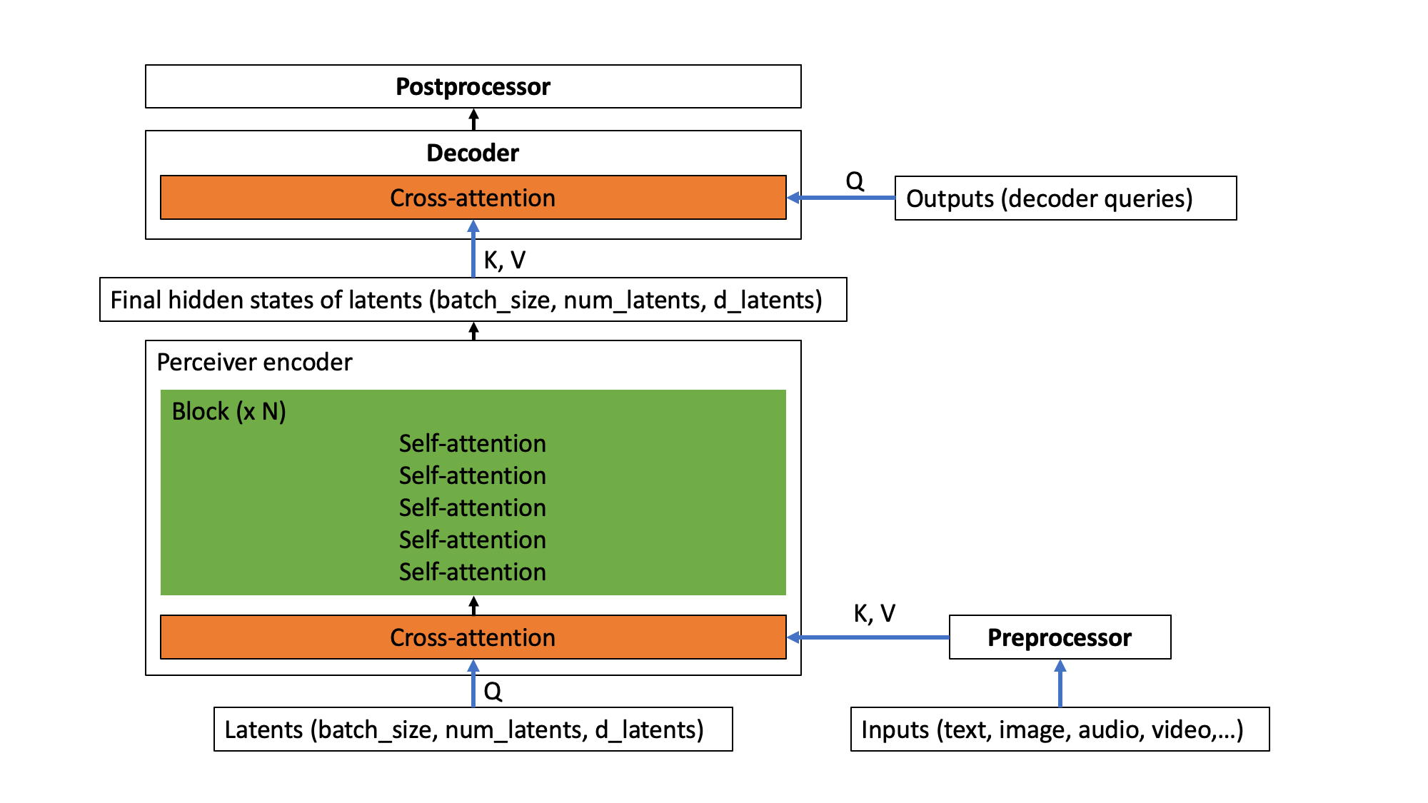
Perceiver 架构。
换句话说,inputs(可以是任意模态或其组合)首先可以通过 preprocessor 进行可选的预处理。接下来,预处理后的输入与 Perceiver 编码器中的 latent 变量执行交叉注意力(cross-attention)操作。在此操作中,latent 变量生成查询(Q),而预处理后的输入生成键和值(KV)。完成此操作后,Perceiver 编码器使用一个(可重复的)自注意力层块来更新 latent 变量的嵌入表示。编码器最终会输出一个形状为 (batch_size, num_latents, d_latents) 的张量,其中包含 latent 变量的最后隐藏状态。随后,有一个可选的 decoder,可用于将 latent 变量的最终隐藏状态解码为更有用的形式,例如分类 logits。这是通过执行交叉注意力操作完成的,其中可训练的嵌入用于生成查询(Q),而 latent 变量用于生成键和值(KV)。最后,还有一个可选的 postprocessor,可用于对 decoder 的输出进行后处理以得到特定特征。
让我们从展示 Perceiver 在文本上的实现方式开始。
用于文本的 Perceiver
假设我们想使用 Perceiver 来执行文本分类任务。由于 Perceiver 的自注意力机制在内存和时间上的需求不依赖于输入的大小,我们可以直接将原始的 UTF-8 字节提供给模型。这样做是有益的,因为常见的基于 Transformer 的模型(如 BERT 和 RoBERTa)都采用了某种形式的显式分词,例如 WordPiece、BPE 或 SentencePiece,而这些方法 可能带来负面影响。为了与 BERT 进行公平比较(BERT 使用的序列长度为 512 个子词 token),作者使用了长度为 2048 字节的输入序列。如果我们再添加一个批次维度,那么模型的 inputs 形状为 (batch_size, 2048)。inputs 包含单段文本的字节 ID(类似于 BERT 的 input_ids)。我们可以使用 PerceiverTokenizer 将文本转换为填充至长度 2048 的字节 ID 序列:
from transformers import PerceiverTokenizer

tokenizer = PerceiverTokenizer.from_pretrained("deepmind/language-perceiver")

text = "hello world"

inputs = tokenizer(text, padding="max_length", return_tensors="pt").input_ids
在这种情况下,我们将 PerceiverTextPreprocessor 作为预处理器提供给模型,它负责将 inputs 嵌入(即将每个字节 ID 转换为对应的向量),并添加绝对位置编码。作为解码器,我们将 PerceiverClassificationDecoder 提供给模型(它将潜在表示的最后隐藏状态转换为分类 logits)。不需要后处理器。换句话说,用于文本分类的 Perceiver 模型(在 HuggingFace Transformers 中称为 PerceiverForSequenceClassification)实现如下:
from torch import nn
from transformers import PerceiverModel
from transformers.models.perceiver.modeling_perceiver import PerceiverTextPreprocessor, PerceiverClassificationDecoder

class PerceiverForSequenceClassification(nn.Module):
    def __init__(self, config):
        super().__init__(config)


> *[注:本文篇幅超长,以上为核心前篇精译,后续内容保留原文呈现]*


self.perceiver = PerceiverModel(
            config,
            input_preprocessor=PerceiverTextPreprocessor(config),
            decoder=PerceiverClassificationDecoder(
                config,
                num_channels=config.d_latents,
                trainable_position_encoding_kwargs=dict(num_channels=config.d_latents, index_dims=1),
                use_query_residual=True,
            ),
        )
One can already see here that the decoder is initialized with trainable position encoding arguments. Why is that? Well, let's take a look in detail at how Perceiver IO works. At initialization, PerceiverModel internally defines a set of latent variables, as follows:
from torch import nn

self.latents = nn.Parameter(torch.randn(config.num_latents, config.d_latents))
In the Perceiver IO paper, one uses 256 latents, and sets the dimensionality of the latents to 1280. If one also adds a batch dimension, the Perceiver has latents of shape (batch_size, 256, 1280). First, the preprocessor (which one provides at initialization) will take care of embedding the UTF-8 byte IDs to embedding vectors. Hence, PerceiverTextPreprocessor will turn the inputs of shape (batch_size, 2048) to a tensor of shape (batch_size, 2048, 768) - assuming that each byte ID is turned into a vector of size 768 (this is determined by the d_model attribute of PerceiverConfig).
After this, Perceiver IO applies cross-attention between the latents (which produce queries) of shape (batch_size, 256, 1280) and the preprocessed inputs (which produce keys and values) of shape (batch_size, 2048, 768). The output of this initial cross-attention operation is a tensor that has the same shape as the queries (which are the latents, in this case). In other words, the output of the cross-attention operation is of shape (batch_size, 256, 1280).
Next, a (repeatable) block of self-attention layers is applied to update the representations of the latents. Note that these don't depend on the length of the inputs (i.e. the bytes) one provided, as these were only used during the cross-attention operation. In the Perceiver IO paper, a single block of 26 self-attention layers (each of which has 8 attention heads) were used to update the representations of the latents of the text model. Note that the output after these 26 self-attention layers still has the same shape as what one initially provided as input to the encoder: (batch_size, 256, 1280). These are also called the "last hidden states" of the latents. This is very similar to the "last hidden states" of the tokens one provides to BERT.
Ok, so now one has final hidden states of shape (batch_size, 256, 1280). Great, but one actually wants to turn these into classification logits of shape (batch_size, num_labels). How can we make the Perceiver output these?
This is handled by PerceiverClassificationDecoder. The idea is very similar to what was done when mapping the inputs to the latent space: one uses cross-attention. But now, the latent variables will produce keys and values, and one provides a tensor of whatever shape we'd like - in this case we'll provide a tensor of shape (batch_size, 1, num_labels) which will act as queries (the authors refer to these as "decoder queries", because they are used in the decoder). This tensor will be randomly initialized at the beginning of training, and trained end-to-end. As one can see, one just provides a dummy sequence length dimension of 1. Note that the output of a QKV attention layer always has the same shape as the shape of the queries - hence the decoder will output a tensor of shape (batch_size, 1, num_labels). The decoder then simply squeezes this tensor to have shape (batch_size, num_labels) and boom, one has classification logits1.
Great, isn't it? The Perceiver authors also show that it is straightforward to pre-train the Perceiver for masked language modeling, similar to BERT. This model is also available in HuggingFace Transformers, and called PerceiverForMaskedLM. The only difference with PerceiverForSequenceClassification is that it doesn't use PerceiverClassificationDecoder as decoder, but rather PerceiverBasicDecoder, to decode the latents to a tensor of shape (batch_size, 2048, 1280). After this, a language modeling head is added, which turns it into a tensor of shape (batch_size, 2048, vocab_size). The vocabulary size of the Perceiver is only 262, namely the 256 UTF-8 byte IDs, as well as 6 special tokens. By pre-training the Perceiver on English Wikipedia and C4, the authors show that it is possible to achieve an overall score of 81.8 on GLUE after fine-tuning.
Perceiver for images
Now that we've seen how to apply the Perceiver to perform text classification, it is straightforward to apply the Perceiver to do image classification. The only difference is that we'll provide a different preprocessor to the model, which will embed the image inputs. The Perceiver authors actually tried out 3 different ways of preprocessing:
- flattening the pixel values, applying a convolutional layer with kernel size 1 and adding learned absolute 1D position embeddings.
- flattening the pixel values and adding fixed 2D Fourier position embeddings.
- applying a 2D convolutional + maxpool layer and adding fixed 2D Fourier position embeddings.
Each of these are implemented in the Transformers library, and called PerceiverForImageClassificationLearned, PerceiverForImageClassificationFourier and PerceiverForImageClassificationConvProcessing respectively. They only differ in their configuration of PerceiverImagePreprocessor. Let's take a closer look at PerceiverForImageClassificationLearned. It initializes a PerceiverModel as follows:
from torch import nn
from transformers import PerceiverModel
from transformers.models.perceiver.modeling_perceiver import PerceiverImagePreprocessor, PerceiverClassificationDecoder

class PerceiverForImageClassificationLearned(nn.Module):
    def __init__(self, config):
        super().__init__(config)

self.perceiver = PerceiverModel(
            config,
            input_preprocessor=PerceiverImagePreprocessor(
                config,
                prep_type="conv1x1",
                spatial_downsample=1,
                out_channels=256,
                position_encoding_type="trainable",
                concat_or_add_pos="concat",
                project_pos_dim=256,
                trainable_position_encoding_kwargs=dict(num_channels=256, index_dims=config.image_size ** 2),
            ),
            decoder=PerceiverClassificationDecoder(
                config,
                num_channels=config.d_latents,
                trainable_position_encoding_kwargs=dict(num_channels=config.d_latents, index_dims=1),
                use_query_residual=True,
            ),
        )
One can see that PerceiverImagePreprocessor is initialized with prep_type = "conv1x1" and that one adds arguments for the trainable position encodings. So how does this preprocessor work in detail? Suppose that one provides a batch of images to the model. Let's say one applies center cropping to a resolution of 224 and normalization of the color channels first, such that the inputs are of shape (batch_size, num_channels, height, width) = (batch_size, 3, 224, 224). One can use PerceiverImageProcessor for this, as follows:
from transformers import PerceiverImageProcessor
import requests
from PIL import Image

processor = PerceiverImageProcessor.from_pretrained("deepmind/vision-perceiver")

url = 'http://images.cocodataset.org/val2017/000000039769.jpg'
image = Image.open(requests.get(url, stream=True).raw)

inputs = processor(image, return_tensors="pt").pixel_values
PerceiverImagePreprocessor (with the settings defined above) will first apply a convolutional layer with kernel size (1, 1) to turn the inputs into a tensor of shape (batch_size, 256, 224, 224) - hence increasing the channel dimension. It will then place the channel dimension last - so now one has a tensor of shape (batch_size, 224, 224, 256). Next, it flattens the spatial (height + width) dimensions such that one has a tensor of shape (batch_size, 50176, 256). Next, it concatenates it with trainable 1D position embeddings. As the dimensionality of the position embeddings is defined to be 256 (see the num_channels argument above), one is left with a tensor of shape (batch_size, 50176, 512). This tensor will be used for the cross-attention operation with the latents.
The authors use 512 latents for all image models, and set the dimensionality of the latents to 1024. Hence, the latents are a tensor of shape (batch_size, 512, 1024) - assuming we add a batch dimension. The cross-attention layer takes the queries of shape (batch_size, 512, 1024) and keys + values of shape (batch_size, 50176, 512) as input, and produces a tensor that has the same shape as the queries, so outputs a new tensor of shape (batch_size, 512, 1024). Next, a block of 6 self-attention layers is applied repeatedly (8 times), to produce final hidden states of the latents of shape (batch_size, 512, 1024). To turn these into classification logits, PerceiverClassificationDecoder is used, which works similarly to the one for text classification: it uses the latents as keys + values, and uses trainable position embeddings of shape (batch_size, 1, num_labels) as queries. The output of the cross-attention operation is a tensor of shape (batch_size, 1, num_labels), which is squeezed to have classification logits of shape (batch_size, num_labels).
The Perceiver authors show that the model is capable of achieving strong results compared to models designed primarily for image classification (such as ResNet or ViT). After large-scale pre-training on JFT, the model that uses conv+maxpool preprocessing (PerceiverForImageClassificationConvProcessing) achieves 84.5 top-1 accuracy on ImageNet. Remarkably, PerceiverForImageClassificationLearned, the model that only employs a 1D fully learned position encoding, achieves a top-1 accuracy of 72.7 despite having no privileged information about the 2D structure of images.
Perceiver for optical flow
The authors show that it's straightforward to make the Perceiver also work on optical flow, which is a decades-old problem in computer vision, with many broader applications. For an introduction to optical flow, I refer to this blog post. Given two images of the same scene (e.g. two consecutive frames of a video), the task is to estimate the 2D displacement for each pixel in the first image. Existing algorithms are quite hand-engineered and complex, however with the Perceiver, this becomes relatively simple. The model is implemented in the Transformers library, and available as PerceiverForOpticalFlow. It is implemented as follows:
from torch import nn
from transformers import PerceiverModel
from transformers.models.perceiver.modeling_perceiver import PerceiverImagePreprocessor, PerceiverOpticalFlowDecoder

class PerceiverForOpticalFlow(nn.Module):
    def __init__(self, config):
        super().__init__(config)

fourier_position_encoding_kwargs_preprocessor = dict(
            num_bands=64,
            max_resolution=config.train_size,
            sine_only=False,
            concat_pos=True,
        )
        fourier_position_encoding_kwargs_decoder = dict(
            concat_pos=True, max_resolution=config.train_size, num_bands=64, sine_only=False
        )

image_preprocessor = PerceiverImagePreprocessor(
            config,
            prep_type="patches",
            spatial_downsample=1,
            conv_after_patching=True,
            conv_after_patching_in_channels=54,
            temporal_downsample=2,
            position_encoding_type="fourier",

fourier_position_encoding_kwargs=fourier_position_encoding_kwargs_preprocessor,
        )

self.perceiver = PerceiverModel(
            config,
            input_preprocessor=image_preprocessor,
            decoder=PerceiverOpticalFlowDecoder(
                config,
                num_channels=image_preprocessor.num_channels,
                output_image_shape=config.train_size,
                rescale_factor=100.0,
                use_query_residual=False,
                output_num_channels=2,
                position_encoding_type="fourier",
                fourier_position_encoding_kwargs=fourier_position_encoding_kwargs_decoder,
            ),
        )
As one can see, PerceiverImagePreprocessor is used as preprocessor (i.e. to prepare the 2 images for the cross-attention operation with the latents) and PerceiverOpticalFlowDecoder is used as decoder (i.e. to decode the final hidden states of the latents to an actual predicted flow). For each of the 2 frames, the authors extract a 3 x 3 patch around each pixel, leading to 3 x 3 x 3 = 27 values for each pixel (as each pixel also has 3 color channels). The authors use a training resolution of (368, 496). If one stacks 2 frames of size (368, 496) of each training example on top of each other, the inputs to the model are of shape (batch_size, 2, 27, 368, 496).
The preprocessor (with the settings defined above) will first concatenate the frames along the channel dimension, leading to a tensor of shape (batch_size, 368, 496, 54) - assuming one also moves the channel dimension to be last. The authors explain in their paper (page 8) why concatenation along the channel dimension makes sense. Next, the spatial dimensions are flattened, leading to a tensor of shape (batch_size, 368*496, 54) = (batch_size, 182528, 54). Then, position embeddings (each of which have dimensionality 258) are concatenated, leading to a final preprocessed input of shape (batch_size, 182528, 322). These will be used to perform cross-attention with the latents.
The authors use 2048 latents for the optical flow model (yes, 2048!), with a dimensionality of 512 for each latent. Hence, the latents have shape (batch_size, 2048, 512). After the cross-attention, one again has a tensor of the same shape (as the latents act as queries). Next, a single block of 24 self-attention layers (each of which has 16 attention heads) are applied to update the embeddings of the latents.
To decode the final hidden states of the latents to an actual predicted flow, PerceiverOpticalFlowDecoder simply uses the preprocessed inputs of shape (batch_size, 182528, 322) as queries for the cross-attention operation. Next, these are projected to a tensor of shape (batch_size, 182528, 2). Finally, one rescales and reshapes this back to the original image size to get a predicted flow of shape (batch_size, 368, 496, 2). The authors claim state-of-the-art results on important benchmarks including Sintel and KITTI when training on AutoFlow, a large synthetic dataset of 400,000 annotated image pairs.
The video below shows the predicted flow on 2 examples.

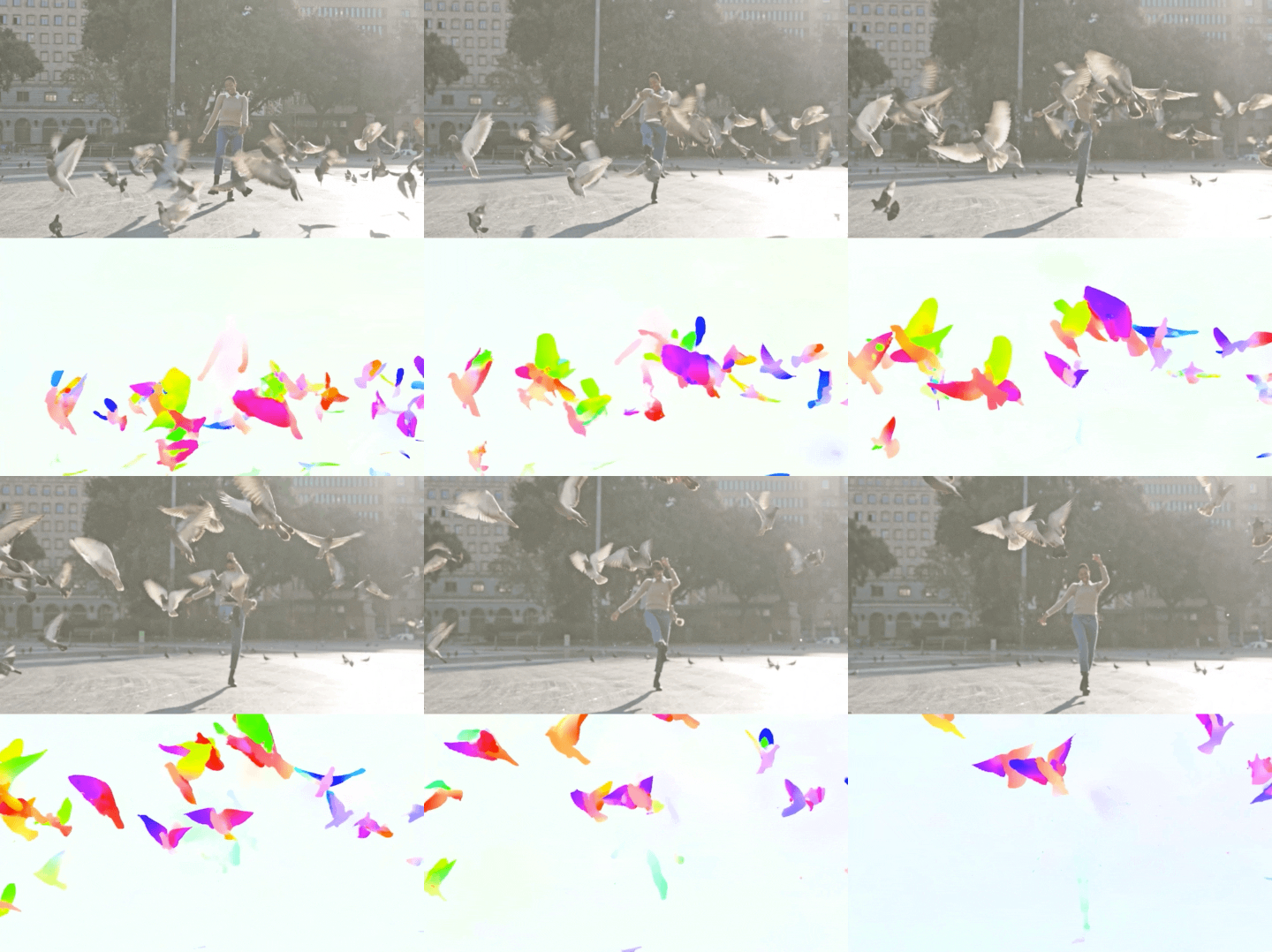
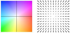
Optical flow estimation by Perceiver IO. The colour of each pixel shows the direction and speed of motion estimated by the model, as indicated by the legend on the right.
Perceiver for multimodal autoencoding
The authors also use the Perceiver for multimodal autoencoding. The goal of multimodal autoencoding is to learn a model that can accurately reconstruct multimodal inputs in the presence of a bottleneck induced by an architecture. The authors train the model on the Kinetics-700 dataset, in which each example consists of a sequence of images (i.e. frames), audio and a class label (one of 700 possible labels). This model is also implemented in HuggingFace Transformers, and available as PerceiverForMultimodalAutoencoding. For brevity, I will omit the code of defining this model, but important to note is that it uses PerceiverMultimodalPreprocessor to prepare the inputs for the model. This preprocessor will first use the respective preprocessor for each modality (image, audio, label) separately. Suppose one has a video of 16 frames of resolution 224x224 and 30,720 audio samples, then the modalities are preprocessed as follows:
- The images - actually a sequence of frames - of shape (batch_size, 16, 3, 224, 224) are turned into a tensor of shape (batch_size, 50176, 243) using
PerceiverImagePreprocessor. This is a “space to depth” transformation, after which fixed 2D Fourier position embeddings are concatenated. - The audio has shape (batch_size, 30720, 1) and is turned into a tensor of shape (batch_size, 1920, 401) using
PerceiverAudioPreprocessor(which concatenates fixed Fourier position embeddings to the raw audio). - The class label of shape (batch_size, 700) is turned into a tensor of shape (batch_size, 1, 700) using
PerceiverOneHotPreprocessor. In other words, this preprocessor just adds a dummy time (index) dimension. Note that one initializes the class label with a tensor of zeros during evaluation, so as to let the model act as a video classifier.
Next, PerceiverMultimodalPreprocessor will pad the preprocessed modalities with modality-specific trainable embeddings to make concatenation along the time dimension possible. In this case, the modality with the highest channel dimension is the class label (it has 700 channels). The authors enforce a minimum padding size of 4, hence each modality will be padded to have 704 channels. They can then be concatenated, hence the final preprocessed input is a tensor of shape (batch_size, 50176 + 1920 + 1, 704) = (batch_size, 52097, 704).
The authors use 784 latents, with a dimensionality of 512 for each latent. Hence, the latents have shape (batch_size, 784, 512). After the cross-attention, one again has a tensor of the same shape (as the latents act as queries). Next, a single block of 8 self-attention layers (each of which has 8 attention heads) is applied to update the embeddings of the latents.
Next, there is PerceiverMultimodalDecoder, which will first create output queries for each modality separately. However, as it is not possible to decode an entire video in a single forward pass, the authors instead auto-encode in chunks. Each chunk will subsample certain index dimensions for every modality. Let's say we process the video in 128 chunks, then the decoder queries will be produced as follows:
- For the image modality, the total size of the decoder query is 16x3x224x224 = 802,816. However, when auto-encoding the first chunk, one subsamples the first 802,816/128 = 6272 values. The shape of the image output query is (batch_size, 6272, 195) - the 195 comes from the fact that fixed Fourier position embeddings are used.
- For the audio modality, the total input has 30,720 values. However, one only subsamples the first 30720/128/16 = 15 values. Hence, the shape of the audio query is (batch_size, 15, 385). Here, the 385 comes from the fact that fixed Fourier position embeddings are used.
- For the class label modality, there's no need to subsample. Hence, the subsampled index is set to 1. The shape of the label output query is (batch_size, 1, 1024). One uses trainable position embeddings (of size 1024) for the queries.
Similarly to the preprocessor, PerceiverMultimodalDecoder pads the different modalities to the same number of channels, to make concatenation of the modality-specific queries possible along the time dimension. Here, the class label has again the highest number of channels (1024), and the authors enforce a minimum padding size of 2, hence every modality will be padded to have 1026 channels. After concatenation, the final decoder query has shape (batch_size, 6272 + 15 + 1, 1026) = (batch_size, 6288, 1026). This tensor produces queries in the cross-attention operation, while the latents act as keys and values. Hence, the output of the cross-attention operation is a tensor of shape (batch_size, 6288, 1026). Next, PerceiverMultimodalDecoder employs a linear layer to reduce the output channels to get a tensor of shape (batch_size, 6288, 512).
Finally, there is PerceiverMultimodalPostprocessor. This class postprocesses the output of the decoder to produce an actual reconstruction of each modality. It first splits up the time dimension of the decoder output according to the different modalities: (batch_size, 6272, 512) for image, (batch_size, 15, 512) for audio and (batch_size, 1, 512) for the class label. Next, the respective postprocessors for each modality are applied:
- The image post processor (which is called
PerceiverProjectionPostprocessorin Transformers) simply turns the (batch_size, 6272, 512) tensor into a tensor of shape (batch_size, 6272, 3) - i.e. it projects the final dimension to RGB values. PerceiverAudioPostprocessorturns the (batch_size, 15, 512) tensor into a tensor of shape (batch_size, 240).PerceiverClassificationPostprocessorsimply takes the first (and only index), to get a tensor of shape (batch_size, 700).
So now one ends up with tensors containing the reconstruction of the image, audio and class label modalities respectively. As one auto-encodes an entire video in chunks, one needs to concatenate the reconstruction of each chunk to have a final reconstruction of an entire video. The figure below shows an example:


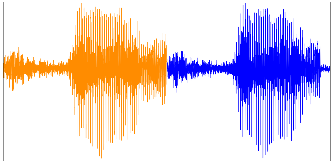
Above: original video (left), reconstruction of the first 16 frames (right). Video taken from the UCF101 dataset. Below: reconstructed audio (taken from the paper).
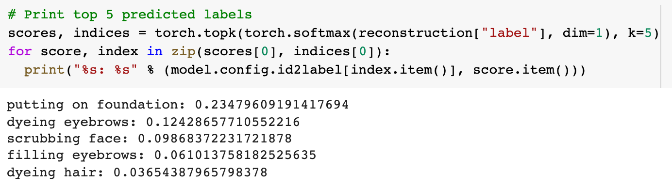
Top 5 predicted labels for the video above. By masking the class label, the Perceiver becomes a video classifier.
With this approach, the model learns a joint distribution across 3 modalities. The authors do note that because the latent variables are shared across modalities and not explicitly allocated between them, the quality of reconstructions for each modality is sensitive to the weight of its loss term and other training hyperparameters. By putting stronger emphasis on classification accuracy, they are able to reach 45% top-1 accuracy while maintaining 20.7 PSNR (peak signal-to-noise ratio) for video.
Other applications of the Perceiver
Note that there are no limits on the applications of the Perceiver! In the original Perceiver paper, the authors showed that the architecture can be used to process 3D point clouds – a common concern for self-driving cars equipped with Lidar sensors. They trained the model on ModelNet40, a dataset of point clouds derived from 3D triangular meshes spanning 40 object categories. The model was shown to achieve a top-1 accuracy of 85.7 % on the test set, competing with PointNet++, a highly specialized model that uses extra geometric features and performs more advanced augmentations.
The authors also used the Perceiver to replace the original Transformer in AlphaStar, the state-of-the-art reinforcement learning system for the complex game of StarCraft II. Without tuning any additional parameters, the authors observed that the resulting agent reached the same level of performance as the original AlphaStar agent, reaching an 87% win-rate versus the Elite bot after behavioral cloning on human data.
It is important to note that the models currently implemented (such as PerceiverForImageClassificationLearned, PerceiverForOpticalFlow) are just examples of what you can do with the Perceiver. Each of these are different instances of PerceiverModel, just with a different preprocessor and/or decoder (and optionally, a postprocessor as is the case for multimodal autoencoding). People can come up with new preprocessors, decoders and postprocessors to make the model solve different problems. For instance, one could extend the Perceiver to perform named-entity recognition (NER) or question-answering similar to BERT, audio classification similar to Wav2Vec2 or object detection similar to DETR.
Conclusion
In this blog post, we went over the architecture of Perceiver IO, an extension of the Perceiver by Google Deepmind, and showed its generality of handling all kinds of modalities. The big advantage of the Perceiver is that the compute and memory requirements of the self-attention mechanism don't depend on the size of the inputs and outputs, as the bulk of compute happens in a latent space (a not-too large set of vectors). Despite its task-agnostic architecture, the model is capabable of achieving great results on modalities such as language, vision, multimodal data, and point clouds. In the future, it might be interesting to train a single (shared) Perceiver encoder on several modalities at the same time, and use modality-specific preprocessors and postprocessors. As Karpathy puts it, it may well be that this architecture can unify all modalities into a shared space, with a library of encoders/decoders.
Speaking of a library, the model is available in HuggingFace Transformers as of today. It will be exciting to see what people build with it, as its applications seem endless!
Appendix
The implementation in HuggingFace Transformers is based on the original JAX/Haiku implementation which can be found here.
The documentation of the Perceiver IO model in HuggingFace Transformers is available here.
Tutorial notebooks regarding the Perceiver on several modalities can be found here.
Footnotes
1 Note that in the official paper, the authors used a two-layer MLP to generate the output logits, which was omitted here for brevity. ↩